AP Calculus AB Unit 7 — Differential Equations Worksheet

All 8 questions

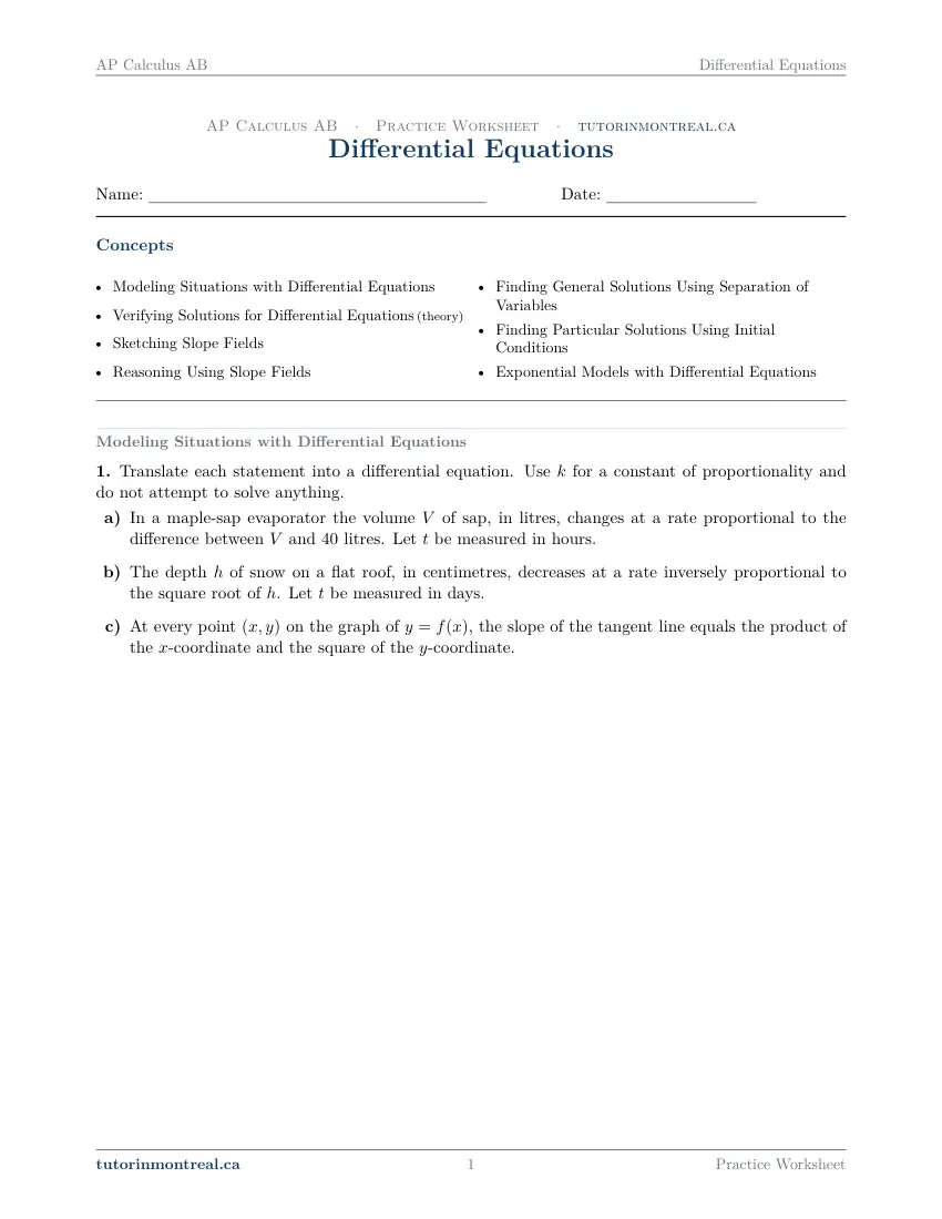
Each question targets one named concept from the sheet. Read them here, or print the PDF — it has working space under each one.

1. Q1Modeling Situations with Differential Equations

   Translate each statement into a differential equation. Use $k$ for a constant of proportionality and do not attempt to solve anything.

   1. In a maple-sap evaporator the volume $V$ of sap, in litres, changes at a rate proportional to the difference between $V$ and $40$ litres. Let $t$ be measured in hours.
   2. The depth $h$ of snow on a flat roof, in centimetres, decreases at a rate inversely proportional to the square root of $h$. Let $t$ be measured in days.
   3. At every point $(x,y)$ on the graph of $y=f(x)$, the slope of the tangent line equals the product of the $x$-coordinate and the square of the $y$-coordinate.
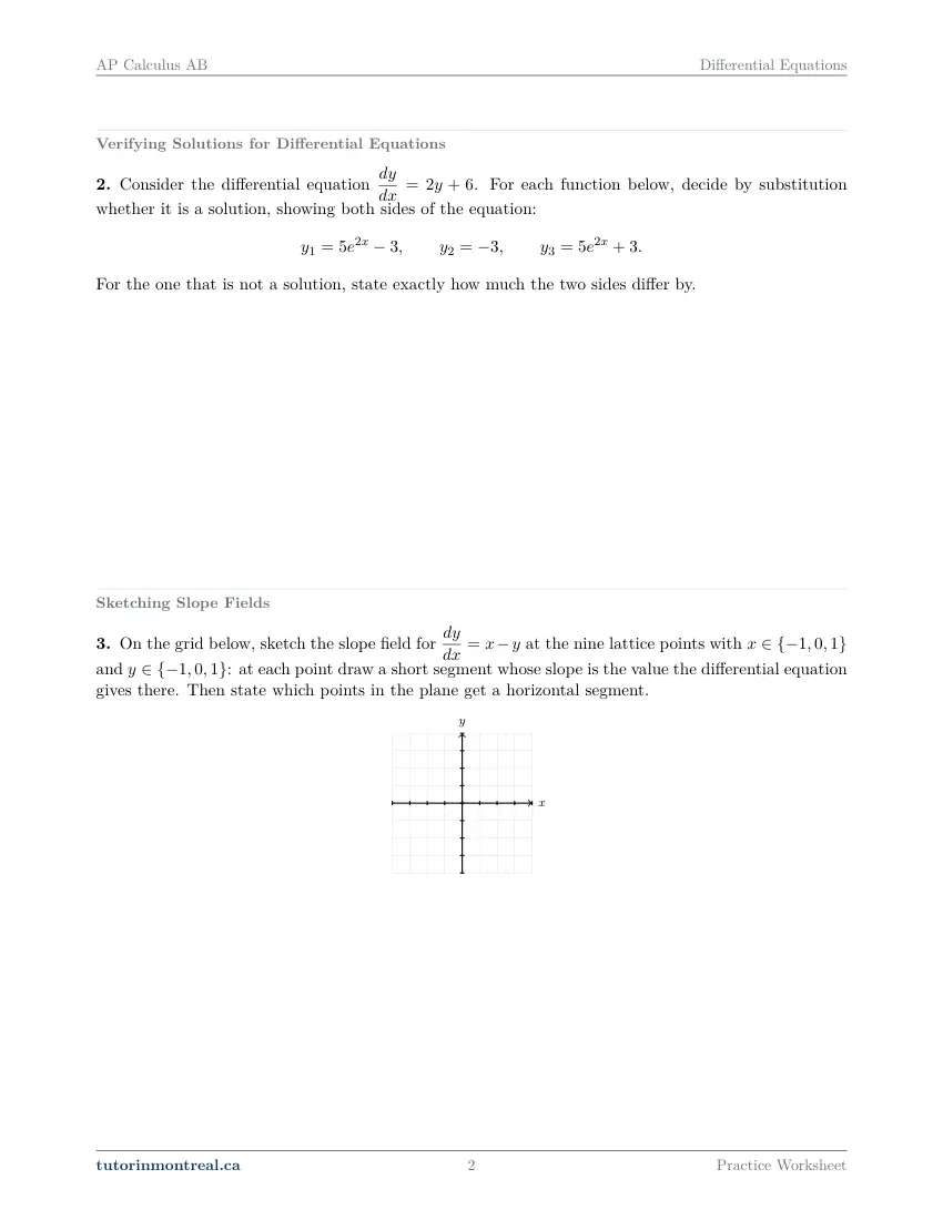
2. Q2Verifying Solutions for Differential Equations

   Consider the differential equation ${\displaystyle \frac{dy}{dx}}=2y+6$. For each function below, decide by substitution whether it is a solution, showing both sides of the equation: $$y_1=5e^{2x}-3,y_2=-3,y_3=5e^{2x}+3.$$ For the one that is not a solution, state exactly how much the two sides differ by.

3. Q3Sketching Slope Fields

   On the grid below, sketch the slope field for ${\displaystyle \frac{dy}{dx}}=x-y$ at the nine lattice points with $x\in \{-1,0,1\}$ and $y\in \{-1,0,1\}$: at each point draw a short segment whose slope is the value the differential equation gives there. Then state which points in the plane get a horizontal segment.

   A blank Cartesian grid for this question is on the printable PDF.

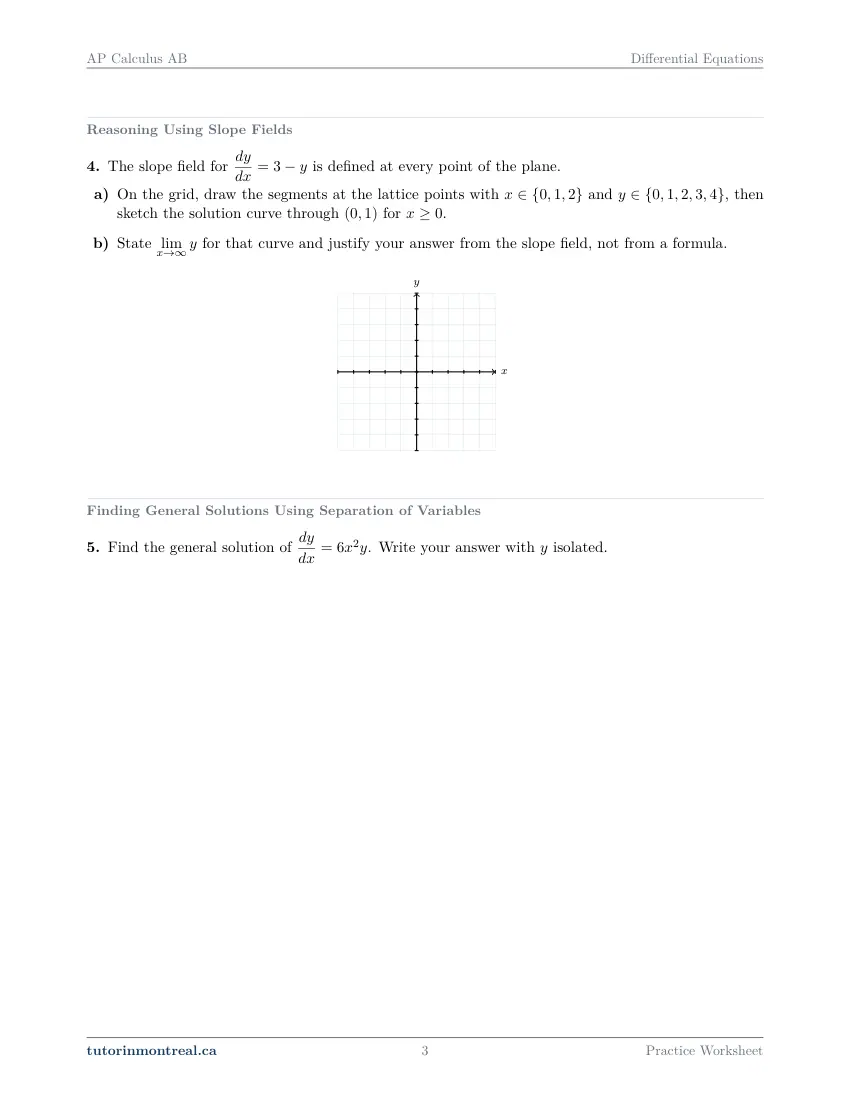
4. Q4Reasoning Using Slope Fields

   The slope field for ${\displaystyle \frac{dy}{dx}}=3-y$ is defined at every point of the plane.

   1. On the grid, draw the segments at the lattice points with $x\in \{0,1,2\}$ and $y\in \{0,1,2,3,4\}$, then sketch the solution curve through $(0,1)$ for $x\ge 0$.
   2. State ${\displaystyle {lim}_{x\to \infty }y}$ for that curve and justify your answer from the slope field, not from a formula.

   A blank Cartesian grid for this question is on the printable PDF.

5. Q5Finding General Solutions Using Separation of Variables

   Find the general solution of ${\displaystyle \frac{dy}{dx}}=6x^{2}y$. Write your answer with $y$ isolated.

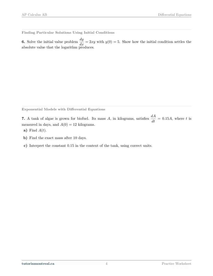
6. Q6Finding Particular Solutions Using Initial Conditions

   Solve the initial value problem ${\displaystyle \frac{dy}{dx}}=2xy$ with $y(0)=5$. Show how the initial condition settles the absolute value that the logarithm produces.

7. Q7Exponential Models with Differential Equations

   A tank of algae is grown for biofuel. Its mass $A$, in kilograms, satisfies ${\displaystyle \frac{dA}{dt}}=0.15A$, where $t$ is measured in days, and $A(0)=12$ kilograms.

   1. Find $A(t)$.
   2. Find the exact mass after $10$ days.
   3. Interpret the constant $0.15$ in the context of the tank, using correct units.
8. Q8Synthesis — drawing on several topics in this unit

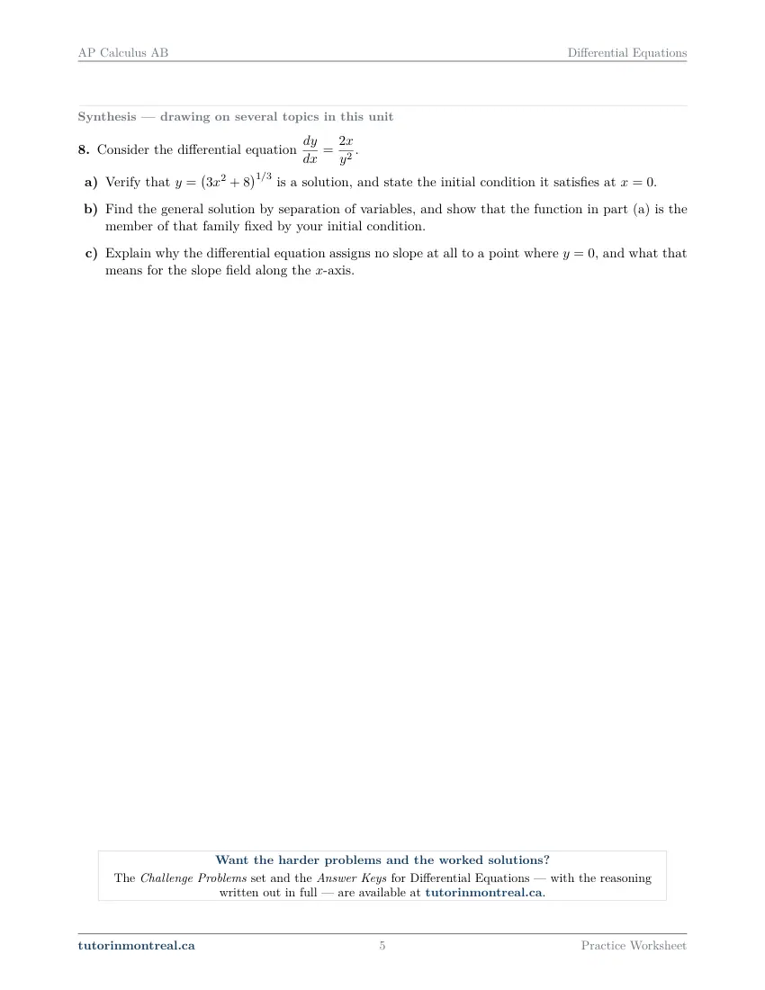
   Consider the differential equation ${\displaystyle \frac{dy}{dx}}={\displaystyle \frac{2x}{y^2}}$.

   1. Verify that $y={(3x^2+8)}^{1/3}$ is a solution, and state the initial condition it satisfies at $x=0$.
   2. Find the general solution by separation of variables, and show that the function in part (a) is the member of that family fixed by your initial condition.
   3. Explain why the differential equation assigns no slope at all to a point where $y=0$, and what that means for the slope field along the $x$-axis.

The 7 challenge problems for this topic are a separate, paid sheet and are not reproduced here.

How to do every concept on this sheet

This is the part worksheet sites usually leave out. Below is the actual reasoning behind each group of questions — not a full solution set, the decisions that get you to one. Read it before you start, or after you get stuck.

Turning a sentence into a differential equation (Q1)

Q1 asks you to translate three descriptions and explicitly tells you not to solve anything. That instruction is the whole point: modelling is a separate skill from solving, and it is tested separately. Translate phrase by phrase, and the equation assembles itself.

Notice what that single equation already knows. When V is above 40, the bracket is positive; when V is below 40, it is negative. So the bracket alone tracks which side of 40 the quantity is on, and the sign of k decides what happens next.

One more habit from Q1: when a model only makes sense on part of the plane, say so. A depth that decreases like k/√h needs h > 0, and the model says nothing at all once the depth reaches zero. Stating the restriction is part of the answer, not decoration.

Verifying a solution — the cheapest mark in the unit (Q2, Q8a)

Q2 hands you three candidate functions for dy/dx = 2y + 6 and asks you to decide which are solutions. There is nothing to solve. A verification is always the same two-column job: differentiate the candidate to get the left side, substitute the candidate into the right side, and compare the two expressions.

Equal for every x, so it is a solution. Write both sides out even when you can see the answer: the mark is for the comparison, and "yes, it works" earns nothing on its own. Two details students lose points on. First, to disprove, a single x where the sides differ is enough — you do not need an identity. Second, when they differ by a constant, say by how much and say that it holds at every x; "they're different" is a weaker statement than the question asked for.

Q8 verifies a solution given implicitly, and there the efficient route is to clear the root first. Faced with y = (3x² + 8)^(1/3), cube both sides to y³ = 3x² + 8 and differentiate that, giving 3y²(dy/dx) = 6x, so dy/dx = 2x/y². Same verification, a third of the algebra, and no chain rule on a fractional power.

Slope fields: the equation gives a slope at every point (Q3)

A differential equation is a rule that turns a point into a slope. Feed it (x, y), out comes dy/dx there. A slope field is nothing more than that rule evaluated at a grid of lattice points and drawn as a short segment at each one. Q3 asks for exactly nine evaluations of dy/dx = x − y, and the discipline is arithmetic, not artistry.

Reading the long run off a slope field, and equilibrium solutions (Q4)

Q4 asks for a limit as x → ∞ and specifically forbids getting it from a formula. That is not an obstacle; it is a faster route, and the argument has three moves.

Two smaller reading skills come with the same territory. When the right side has no x in it, the field is unchanged as you slide left or right, which means any solution curve shifted horizontally is again a solution — the family is one curve and all of its translates. And where the right side is undefined, as dy/dx = 2x/y² is everywhere on the x-axis (Q8), the field has no segment at all: the equation simply declines to say what the slope is there, and a solution reaching that line would have to arrive with a vertical tangent.

Separation of variables, in the order that works (Q5, Q6)

Separation applies when the right side factors into a function of x times a function of y — 6x²y in Q5, 2xy in Q6. Everything with a y goes to the dy side, everything with an x to the dx side, and then you antidifferentiate both sides at once. The steps below are in the order that keeps the algebra clean; the common wreck is doing step 5 before step 4.

When there is no initial condition, as in Q5, you are asked for the general solution and C stays a letter. For dy/dx = 6x²y, separation gives ln|y| = 2x³ + C₁, then |y| = e^(C₁) · e^(2x³), and absorbing the sign into a new constant C leaves y = Ce^(2x³). The question asks for y isolated, so leaving the answer as a logarithm is an incomplete response.

Exponential models, and what k actually means (Q7)

dA/dt = kA is the one differential equation worth knowing by sight. Its solutions are A = A₀e^(kt), where A₀ is the value at t = 0 — you can quote that on the AP exam without deriving it, though separation reproduces it in three lines. Q7 has dA/dt = 0.15A with A(0) = 12, so A(t) = 12e^(0.15t), and the mass at t = 10 is 12e^(1.5) kilograms. When a question says exact, that expression is the answer; replacing it with a decimal is a wrong answer to the question asked.

The same reasoning kills the most common wrong answer in the whole unit: taking an average rate of change over an interval and projecting it forward as if it were constant. In an exponential model the rate is proportional to the amount, so it changes continuously — an average over the first stretch is not a rate that continues. If you are asked when a quantity reaches a value, solve the equation for t; do not divide a total by an average.

Preview all 5 pages

Click any page to open the full PDF.

Getting the most out of it

Do the translation questions without solving anything

Q1 is worth practising alone, cold, on statements you invent. Give yourself thirty seconds per sentence and write only the equation and its restriction. Modelling is a separate exam skill from solving, and it is the one students skip because it looks too easy.

Verify every answer you produce

Q2 and Q8(a) teach a check you should then use everywhere else on the sheet. After solving Q5, Q6 or Q7, differentiate your own answer and substitute it back. It costs a line and it catches sign errors, dropped constants and a mis-solved initial condition.

Say the sign of k out loud before you compute it

Whenever a model has a constant of proportionality, state whether it is positive or negative and why, in one sentence, before touching any algebra. Growing or decaying, toward the equilibrium or away from it — if you can't say it in words, the algebra will not fix that.

Draw the slope field on the printed page, not on scrap

Q3 and Q4 come with a grid in the PDF. Use it: build the table of values first, then draw. And compare your segments with each other when you're done — the steepest and the flattest should be obviously different, because that comparison is what the drawing is marked on.

Common questions