University Linear Algebra — Projections, Least Squares and Symmetric Matrices Worksheet

All 11 questions

Each question targets one named concept from the sheet. Read them here, or print the PDF — it has working space under each one.

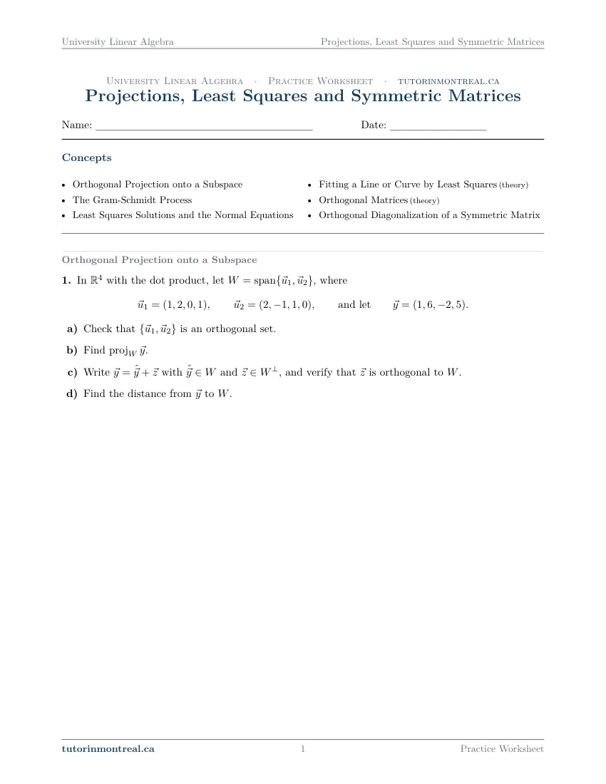
1. Q1Orthogonal Projection onto a Subspace

   In ${ℝ}^4$ with the dot product, let $W=span\{{\overrightarrow{u}}_1,{\overrightarrow{u}}_2\}$, where $${\overrightarrow{u}}_1=(1,2,0,1),{\overrightarrow{u}}_2=(2,-1,1,0),\text{and let}\overrightarrow{y}=(1,6,-2,5).$$

   1. Check that $\{{\overrightarrow{u}}_1,{\overrightarrow{u}}_2\}$ is an orthogonal set.
   2. Find ${proj}_W\overrightarrow{y}$.
   3. Write $\overrightarrow{y}=\widehat{\overrightarrow{y}}+\overrightarrow{z}$ with $\widehat{\overrightarrow{y}}\in W$ and $\overrightarrow{z}\in W^{⟂}$, and verify that $\overrightarrow{z}$ is orthogonal to $W$.
   4. Find the distance from $\overrightarrow{y}$ to $W$.
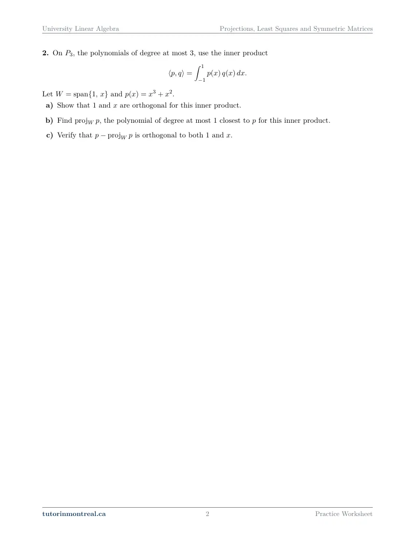
2. Q2Orthogonal Projection onto a Subspace

   On $P_3$, the polynomials of degree at most $3$, use the inner product $$⟨p,q⟩={\int }_{-1}^{1}p(x)q(x)dx.$$ Let $W=span\{1,x\}$ and $p(x)=x^3+x^2$.

   1. Show that $1$ and $x$ are orthogonal for this inner product.
   2. Find ${proj}_{W}p$, the polynomial of degree at most $1$ closest to $p$ for this inner product.
   3. Verify that $p-{proj}_{W}p$ is orthogonal to both $1$ and $x$.
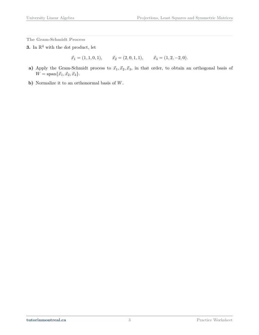
3. Q3The Gram-Schmidt Process

   In ${ℝ}^4$ with the dot product, let $${\overrightarrow{x}}_1=(1,1,0,1),{\overrightarrow{x}}_2=(2,0,1,1),{\overrightarrow{x}}_3=(1,2,-2,0).$$

   1. Apply the Gram-Schmidt process to ${\overrightarrow{x}}_1,{\overrightarrow{x}}_2,{\overrightarrow{x}}_3$, in that order, to obtain an orthogonal basis of $W=span\{{\overrightarrow{x}}_1,{\overrightarrow{x}}_2,{\overrightarrow{x}}_3\}$.
   2. Normalize it to an orthonormal basis of $W$.
4. Q4The Gram-Schmidt Process

   On $P_2$, the polynomials of degree at most $2$, use the inner product $$⟨p,q⟩=p(0)q(0)+p(1)q(1)+p(2)q(2).$$

   1. Apply the Gram-Schmidt process to the basis $\{1,x,x^2\}$, in that order.
   2. Normalize the result to an orthonormal basis of $P_2$ for this inner product.
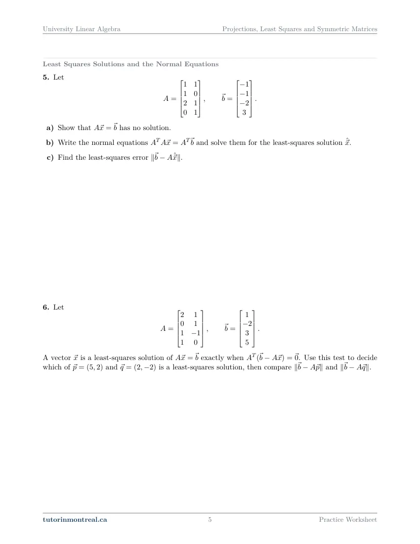
5. Q5Least Squares Solutions and the Normal Equations

   Let $$A=\left[\begin{array}{cc}1& 1\\ 1& 0\\ 2& 1\\ 0& 1\end{array}\right],\overrightarrow{b}=\left[\begin{array}{c}-1\\ -1\\ -2\\ 3\end{array}\right].$$

   1. Show that $A\overrightarrow{x}=\overrightarrow{b}$ has no solution.
   2. Write the normal equations $A^{T}A\overrightarrow{x}=A^T\overrightarrow{b}$ and solve them for the least-squares solution $\widehat{\overrightarrow{x}}$.
   3. Find the least-squares error $\Vert \overrightarrow{b}-A\widehat{\overrightarrow{x}}\Vert$.
6. Q6Least Squares Solutions and the Normal Equations

   Let $$A=\left[\begin{array}{cc}2& 1\\ 0& 1\\ 1& -1\\ 1& 0\end{array}\right],\overrightarrow{b}=\left[\begin{array}{c}1\\ -2\\ 3\\ 5\end{array}\right].$$ A vector $\overrightarrow{x}$ is a least-squares solution of $A\overrightarrow{x}=\overrightarrow{b}$ exactly when $A^T(\overrightarrow{b}-A\overrightarrow{x})=\overrightarrow{0}$. Use this test to decide which of $\overrightarrow{p}=(5,2)$ and $\overrightarrow{q}=(2,-2)$ is a least-squares solution, then compare $\Vert \overrightarrow{b}-A\overrightarrow{p}\Vert$ and $\Vert \overrightarrow{b}-A\overrightarrow{q}\Vert$.

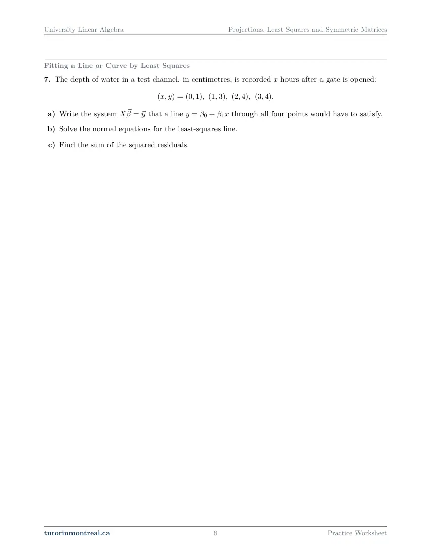
7. Q7Fitting a Line or Curve by Least Squares

   The depth of water in a test channel, in centimetres, is recorded $x$ hours after a gate is opened: $$(x,y)=(0,1),(1,3),(2,4),(3,4).$$

   1. Write the system $X\overrightarrow{\beta }=\overrightarrow{y}$ that a line $y={\beta }_0+{\beta }_{1}x$ through all four points would have to satisfy.
   2. Solve the normal equations for the least-squares line.
   3. Find the sum of the squared residuals.
8. Q8Orthogonal Matrices

   A square matrix $Q$ is orthogonal when $Q^{T}Q=I$. Decide which of the following matrices are orthogonal, and give the inverse of each one that is. $$M_1=\frac{1}{2}\left[\begin{array}{cccc}1& 1& 1& 1\\ 1& -1& 1& -1\\ 1& 1& -1& -1\\ -1& 1& 1& -1\end{array}\right],M_2=\left[\begin{array}{cc}1& 2\\ -2& 1\end{array}\right],M_3=\frac{1}{3}\left[\begin{array}{cc}2& 1\\ 2& -2\\ 1& 2\end{array}\right],M_4=\left[\begin{array}{ccc}0& 0& 1\\ 1& 0& 0\\ 0& 1& 0\end{array}\right].$$

9. Q9Orthogonal Diagonalization of a Symmetric Matrix

   Orthogonally diagonalize $$A=\left[\begin{array}{ccc}1& 2& 0\\ 2& 2& 2\\ 0& 2& 3\end{array}\right]:$$ find an orthogonal matrix $P$ and a diagonal matrix $D$ with $A=PD{P}^T$.

10. Q10Orthogonal Diagonalization of a Symmetric Matrix

    The symmetric matrix $$A=\left[\begin{array}{cccc}1& -1& -1& -1\\ -1& 1& -1& -1\\ -1& -1& 1& -1\\ -1& -1& -1& 1\end{array}\right]$$ has eigenvalues $-2$ and $2$ only. Find a basis of each eigenspace, and then an orthogonal matrix $P$ and a diagonal matrix $D$ with $A=PD{P}^T$.

11. Q11Synthesis — drawing on several topics in this unit

    A technician codes four equally spaced times as $x=-3,-1,1,3$ and reads a voltage $y$, in millivolts, at each: $y=1,2,4,7$. The least-squares line $y={\beta }_0+{\beta }_{1}x$ is wanted.

    1. Write the design matrix $X$ and show that its two columns are orthogonal.
    2. Use orthogonal projection onto $Col(X)$ to find the fitted values $\widehat{\overrightarrow{y}}$, and read off ${\beta }_0$ and ${\beta }_1$.
    3. Confirm the line with the normal equations, and find the sum of the squared residuals.

The 8 challenge problems for this topic are a separate, paid sheet and are not reproduced here.

The rest of this unit

The worksheet is the practice, and it is free. Two more printable documents cover the same unit and come with the University Linear Algebra bundle: read the notes first, work this sheet, then sit the test closed-book. See what each one covers.

What the Projections, Least Squares and Symmetric Matrices notes cover  About the Projections, Least Squares and Symmetric Matrices unit test

How to do every concept on this sheet

This is the part worksheet sites usually leave out. Below is the actual reasoning behind each group of questions — not a full solution set, the decisions that get you to one. Read it before you start, or after you get stuck.

Orthogonal projection onto a subspace

Given an orthogonal basis of a subspace W, the projection of y onto W is the sum of its projections onto each basis vector — the same ratios of inner products as the coordinates in the previous set.

Q1 walks through the whole idea in four-space. Part (a) checks the hypothesis — the formula above is only valid for an orthogonal basis. Part (b) applies it. Part (c) splits y into the piece in W and the piece orthogonal to W, and asks you to verify the second piece really is orthogonal: take its dot product with each spanning vector. Part (d) uses the reason projections matter.

Q2 is the same formula on cubic polynomials, with the integral inner product. The subspace is the polynomials of degree at most 1, and the projection is the best approximation to the cubic among straight lines, in the sense that inner product measures. Part (a) checks that 1 and x are orthogonal; symmetry of the interval makes that, and much of part (b), short. Part (c) is the check from Q1(c).

The Gram-Schmidt process

Gram-Schmidt turns any basis into an orthogonal one spanning the same space, one vector at a time: keep the first, and from each later vector subtract its projection onto the span of the ones already built.

Q3 applies the process in four-space; Q4 applies it to 1, x, x² with an inner product built from values at three points. The steps are identical — only the inner product changes. Every inner product in Q4 is a sum of three products, so write down the values of each polynomial at 0, 1 and 2 once and reuse them.

Least squares and the normal equations

When Ax = b has no solution, the best you can do is make Ax as close to b as possible. The closest vector of the column space to b is its projection, and the x that produces it satisfies the normal equations.

Q5 goes through the full procedure. Part (a) shows the system is inconsistent — reduce the augmented matrix and point to the offending row. Part (b) forms the 2 × 2 matrix AᵀA and the vector Aᵀb, and solves. Part (c) measures how far off the best answer still is: compute the residual vector b − Ax̂ and its length.

Q6 gives the test in its orthogonality form and two candidates. For each, compute the residual b − Ax and multiply by Aᵀ; the least-squares solution is the one for which the product is the zero vector. Comparing the two residual lengths afterwards shows the closest-point property in numbers.

Fitting a line to data

Q7 records four measurements and asks for the least-squares line. A line through all four points would have to satisfy four equations in two unknowns — the intercept and the slope. Each row of the design matrix X is a 1 followed by an x-value; the right-hand side is the list of y-values.

Orthogonal matrices

A square matrix is orthogonal when its transpose times itself is the identity — equivalently, when its columns form an orthonormal set. Then its inverse is its transpose, with no computation. Q8 gives four matrices to classify.

Orthogonal diagonalization of a symmetric matrix

A real symmetric matrix can always be diagonalized by an orthogonal matrix — this is the spectral theorem, and it is where the course ends. Its eigenvalues are real, and eigenvectors for different eigenvalues are automatically orthogonal.

Q9 is a 3 × 3 symmetric matrix. Find the eigenvalues and an eigenvector for each, check that the eigenvectors are orthogonal, normalise them, and use them as the columns of P. Because P is orthogonal, the formula uses Pᵀ, not P⁻¹.

Q10 gives a 4 × 4 symmetric matrix with only two eigenvalues, so at least one eigenspace has dimension more than one. Eigenvectors from different eigenspaces are orthogonal for free; inside one eigenspace they are not, and a basis found by row reduction usually is not orthogonal.

The synthesis question

Q11 fits a line to four measurements whose x-values are symmetric about zero. Part (a) writes the design matrix, as in Q7, and shows its two columns are orthogonal — the symmetric x-values are why. Part (b) uses that orthogonality: project y onto the column space with Q1's formula, and read the two coefficients straight off the projection, since the fitted values are the intercept times one column plus the slope times the other. Part (c) confirms the same line by Q5's normal equations and finds the sum of squared residuals.

Preview all 10 pages

Click any page to open the full PDF.

Getting the most out of it

Check orthogonality before you use a formula that needs it

The projection formula and the coordinate formula both assume an orthogonal basis. One line of dot products before you start saves a whole wrong answer.

Verify every projection

After projecting, compute y minus the projection and take its inner product with each spanning vector of W. Every one must be zero. The same check confirms a least-squares solution: Aᵀ times the residual is zero.

Clear fractions during Gram-Schmidt, normalise at the end

Rescaling intermediate vectors is free and keeps the numbers small. Square roots belong only in the final normalising step.

For symmetric matrices, count dimensions per eigenvalue

Before building P, note which eigenspaces have dimension more than one. Those are the only places Gram-Schmidt is needed, and forgetting it there is the usual reason P fails to be orthogonal.

Common questions