University Introductory Statistics — Descriptive Statistics Worksheet

5 of the 9 questions

Each question targets one named concept from the sheet. Read them here, or print the PDF — it has working space under each one. 5 of the 9 questions are printed below. The other 4 are built on a diagram or a table of values that does not translate to the page, so they are in the free PDF — marked below where they would have come.

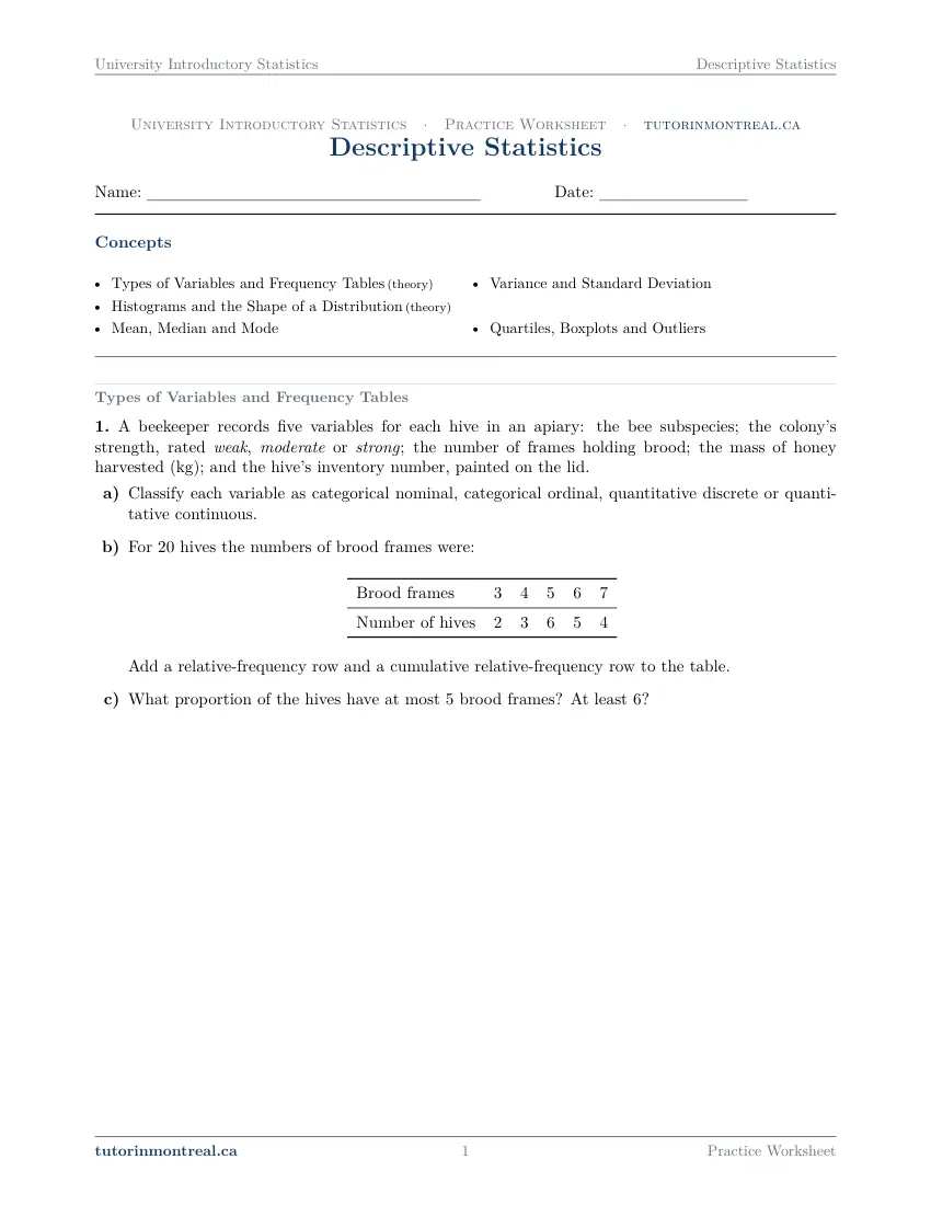
1. Q1Types of Variables and Frequency Tables

   This question is built around a diagram or a table of values. Open it in the PDF.

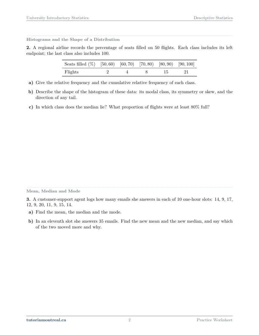
2. Q2Histograms and the Shape of a Distribution

   This question is built around a diagram or a table of values. Open it in the PDF.

3. Q3Mean, Median and Mode

   A customer-support agent logs how many emails she answers in each of $10$ one-hour slots: $14$, $9$, $17$, $12$, $9$, $20$, $11$, $9$, $15$, $14$.

   1. Find the mean, the median and the mode.
   2. In an eleventh slot she answers $35$ emails. Find the new mean and the new median, and say which of the two moved more and why.
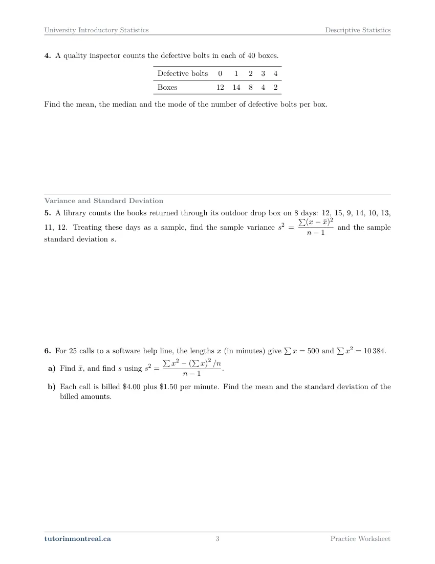
4. Q4Mean, Median and Mode

   This question is built around a diagram or a table of values. Open it in the PDF.

5. Q5Variance and Standard Deviation

   A library counts the books returned through its outdoor drop box on $8$ days: $12$, $15$, $9$, $14$, $10$, $13$, $11$, $12$. Treating these days as a sample, find the sample variance $s^2={\displaystyle \frac{\sum (x-\overline{x}{)}^2}{n-1}}$ and the sample standard deviation $s$.

6. Q6Variance and Standard Deviation

   For $25$ calls to a software help line, the lengths $x$ (in minutes) give $\sum x=500$ and $\sum x^2=10384$.

   1. Find $\overline{x}$, and find $s$ using $s^2={\displaystyle \frac{\sum x^2-{(\sum x)}^2/n}{n-1}}$.
   2. Each call is billed $4.00 plus $1.50 per minute. Find the mean and the standard deviation of the billed amounts.
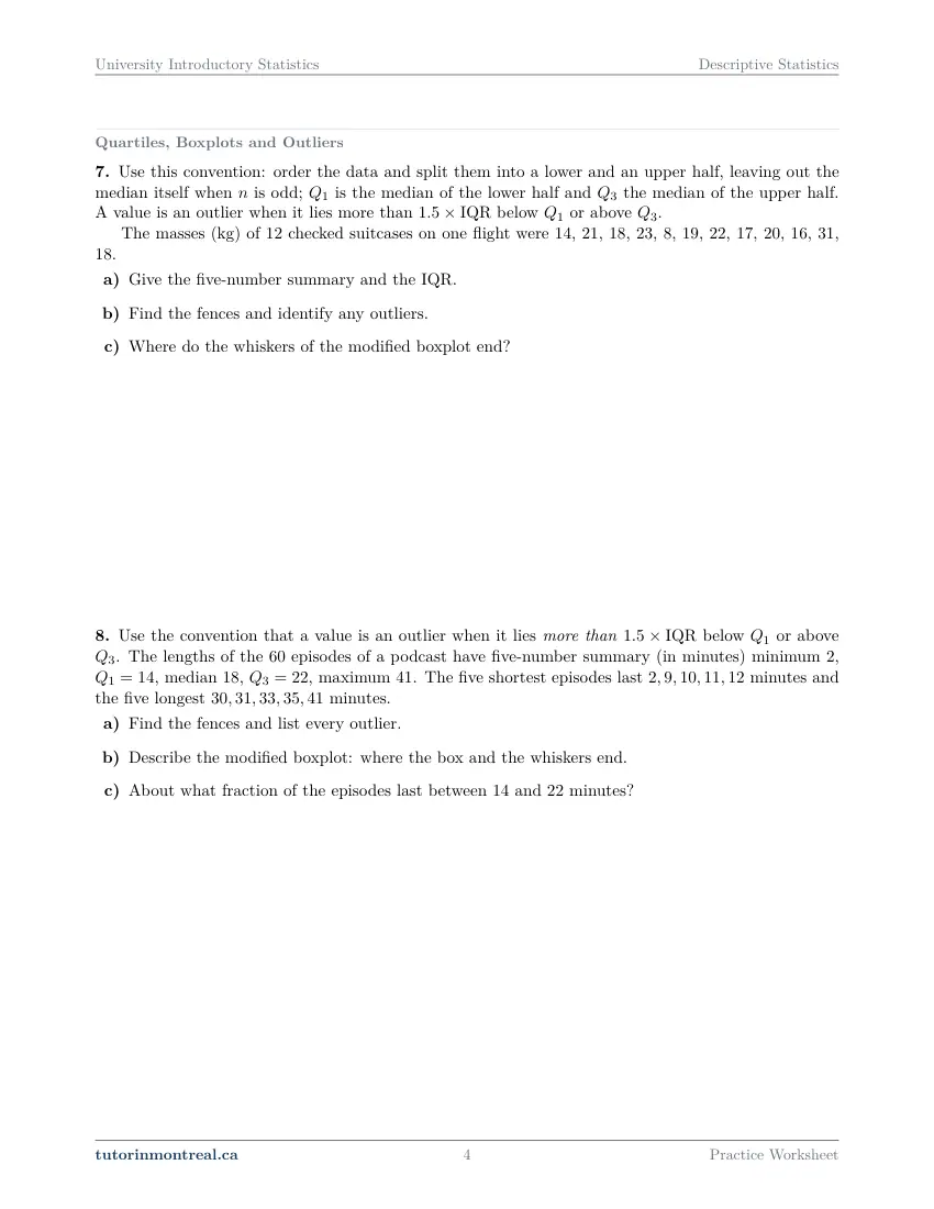
7. Q7Quartiles, Boxplots and Outliers

   Use this convention: order the data and split them into a lower and an upper half, leaving out the median itself when $n$ is odd; $Q_1$ is the median of the lower half and $Q_3$ the median of the upper half. A value is an outlier when it lies more than $1.5\times \text{IQR}$ below $Q_1$ or above $Q_3$.

   The masses (kg) of $12$ checked suitcases on one flight were $14$, $21$, $18$, $23$, $8$, $19$, $22$, $17$, $20$, $16$, $31$, $18$.

   1. Give the five-number summary and the IQR.
   2. Find the fences and identify any outliers.
   3. Where do the whiskers of the modified boxplot end?
8. Q8Quartiles, Boxplots and Outliers

   Use the convention that a value is an outlier when it lies more than $1.5\times \text{IQR}$ below $Q_1$ or above $Q_3$. The lengths of the $60$ episodes of a podcast have five-number summary (in minutes) minimum $2$, $Q_1=14$, median $18$, $Q_3=22$, maximum $41$. The five shortest episodes last $2,9,10,11,12$ minutes and the five longest $30,31,33,35,41$ minutes.

   1. Find the fences and list every outlier.
   2. Describe the modified boxplot: where the box and the whiskers end.
   3. About what fraction of the episodes last between $14$ and $22$ minutes?
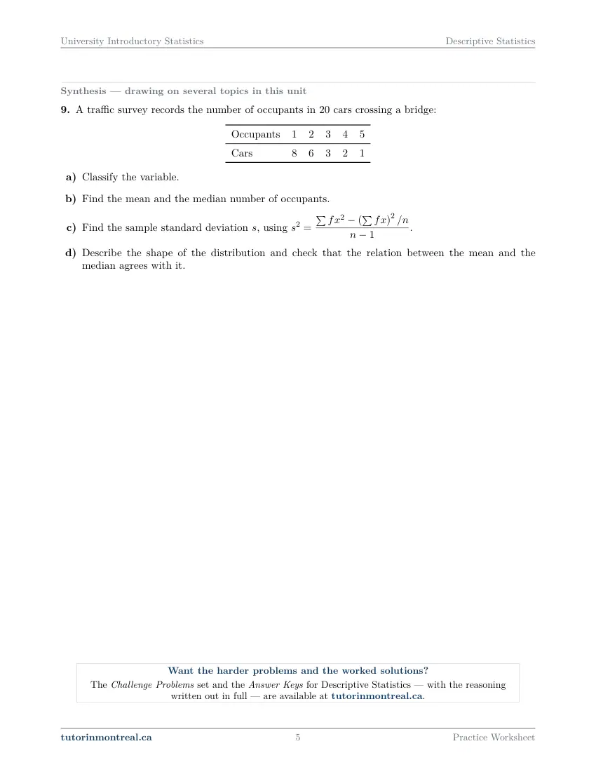
9. Q9Synthesis — drawing on several topics in this unit

   This question is built around a diagram or a table of values. Open it in the PDF.

The 6 challenge problems for this topic are a separate, paid sheet and are not reproduced here.

How to do every concept on this sheet

This is the part worksheet sites usually leave out. Below is the actual reasoning behind each group of questions — not a full solution set, the decisions that get you to one. Read it before you start, or after you get stuck.

Types of variables

Before any arithmetic, decide what kind of thing each column holds — because the kind decides which summaries are even legal. A mean of a set of labels is meaningless however neatly the labels are written as numerals.

Frequency, relative frequency and cumulative relative frequency

A frequency table is three rows once it is finished. The frequency f counts how many observations took each value; the relative frequency is f/n, the share of the data at that value; and the cumulative relative frequency adds the relative frequencies from the left, accumulating as it goes.

Q1(b) asks for both extra rows on a table of counts, and Q2(a) asks for the same two rows on a table of classes. Work with the same n throughout — add the frequency row first and use that total, rather than the total printed in the sentence above the table, so that a misread figure shows up immediately.

Q1(c) then reads two proportions off the finished table, and the wording is the whole exercise. "At most 5" means 5 and everything below it, so it is a cumulative entry read directly. "At least 6" means 6 and everything above it, which the cumulative row does not hold — take it as 1 minus the cumulative entry just below, or add the remaining relative frequencies and check that the two routes agree.

Histograms and the shape of a distribution

Q2 works from classes rather than single values, and the question states the endpoint convention it wants: each class includes its left endpoint, and the last class is closed at the top so that nothing falls outside the table. Use the stated convention and do not import a different one — a value sitting exactly on a boundary has to land in exactly one class.

Q2(b) asks for three things about the picture, and each has a definite meaning:

Q2(c) sends you back to the cumulative row for two different jobs. To find the class holding the median, run along the cumulative relative frequencies until they first reach 0.5 — the class where that happens is the one the middle observation falls in, and with grouped data that class is the whole answer, since the individual values are no longer visible. The proportion at or above a class boundary is then the sum of the relative frequencies of the classes above it, or 1 minus the cumulative entry at that boundary; the second route is shorter and the first is the check on it.

Mean, median and mode

Three measures of centre, three different questions answered. The mean is the balance point and uses the size of every value; the median is the positional middle and uses only the order; the mode is the value that occurs most often and is the only one of the three that also works on categories.

Q3 gives ten values as a plain list. Order them before looking for the median — when n is even the median sits halfway between the two middle entries of the sorted list, and when n is odd it is the single middle entry. The mode needs no ordering, only a tally, and a list can have no mode at all or more than one.

Q4 is the same three measures read out of a frequency table, which is a different piece of arithmetic for each. The mean is Σfx/Σf: multiply each value by its frequency, add the products, divide by the total count — not by the number of distinct values, which is the standard error here. The median is positional, so build a cumulative count and find which value the middle observation lands on; with n even, locate both middle positions and check whether they fall on the same value. The mode is the value carrying the largest frequency, which you read off the table with no arithmetic at all.

Variance and standard deviation

Spread is measured from the mean outwards. The deviation of a value is x − x̄; the deviations always add to zero, so they are squared before being averaged, and the sample version divides by n − 1 rather than n. The standard deviation s is the square root of that, which puts the answer back into the units of the data.

Q5 wants the definitional route on eight values, and it is worth laying out as a table with a column for x, a column for x − x̄ and a column for (x − x̄)². Add the middle column before going further: it must come to zero, and if it does not the mean is wrong and nothing after it can be right.

Q6 hands you Σx and Σx² for twenty-five observations and no list at all, which is exactly the situation the computational formula exists for. It is the same quantity as the definitional one, rearranged so that it needs only the two sums.

Q6(b) is a linear transformation: each observation is charged a fixed amount plus a fixed rate per minute, so the billed amount is a + bx for constants a and b read out of the sentence. The two summaries do not behave alike under it. Adding a constant shifts every value by the same amount, so no two observations move apart and the spread is untouched while the centre slides; multiplying by a constant stretches the distances between observations as well, so it scales both summaries.

So there is no need to rebuild anything from the data: identify a and b, apply the two rules, and state the units of the results. Doing it this way is also the check — a fixed charge that changed the standard deviation would mean the wrong rule was applied.

Quartiles, boxplots and outliers

Q7 opens by stating the convention it wants, and that matters: there are several defensible ways to split a data set into quarters and they can disagree by a whole value. Use the one written into the question. Order the data, cut the ordered list in half — leaving the median itself out when n is odd — and take Q₁ as the median of the lower half and Q₃ as the median of the upper half. (Those subscripted Q's are quartiles; Q7 and Q8 are question numbers.)

Q8 reverses the supply of information: the five-number summary is given for sixty observations you never see, along with the five smallest and the five largest. Everything you need is still there. The quartiles give the IQR and the fences; then the outliers can only be among the listed extremes, because every unlisted value lies between the fifth smallest and the fifth largest. Compare each listed extreme with its fence and stop when you reach one that is inside — the ones beyond it are inside too, since the list is in order.

The synthesis question

Q9 runs the whole sheet on one small frequency table. Part (a) is the classification of Q1 again — apply the same two questions from the tree above. Parts (b) and (c) are the frequency-table versions of the mean, the median and the standard deviation, so Σfx and Σfx² are the columns to build; the formula printed in the question is the computational one from Q6 with f carried through, and the trap from Q4 applies here too, since the values being summarized are the counts of occupants and not the counts of cars.

Part (d) is the one that ties the set together. Describe the shape from the table as you described it from the histogram in Q2, then check it against the relation between the two measures of centre you have just computed. The general rule is that a long tail pulls the mean towards it while the median stays put, so in a right-skewed distribution the mean sits above the median, in a left-skewed one below it, and in a roughly symmetric one the two are close. State the rule, state which side your mean fell on, and say whether the two descriptions agree — the agreement is the answer, not either half on its own.

Preview all 5 pages

Click any page to open the full PDF.

Getting the most out of it

Sort first, always

The median, the quartiles, the five-number summary and both boxplots are positional: they are statements about where a value sits in the ordered list, and every one of them is wrong if the list is not sorted. Write the ordered list out once, on its own line, and work from it for the rest of the question.

Keep the whole number until the last line

A mean rounded before it is used again is the most common source of a nearly-right standard deviation. Carry every digit through the intermediate steps and round once, at the end, to a sensible number of decimals — one more than the data usually does.

Make each table prove itself

Relative frequencies add to 1; a cumulative row ends at 1; deviations from the mean add to zero; Σf is the same n you divided by. Each of these takes ten seconds and each one catches a whole class of arithmetic slip before it propagates into the next part of the question.

Say what every number means, with its units

This course asks for interpretation beside computation, so a part that ends at a bare number is unfinished. A standard deviation is a typical distance from the mean in the units of the data; a variance is in squared units; a relative frequency is a share of the whole. Write the sentence, not just the figure.

Describe a distribution in the same three words every time

Shape, centre, spread — and outliers if there are any. Practising that order on Q2, Q7 and Q9 means that when a later set asks whether a procedure is safe to use, you are already looking at the three things that decide it.

Common questions