University Introductory Statistics — Hypothesis Tests Worksheet

All 14 questions

Each question targets one named concept from the sheet. Read them here, or print the PDF — it has working space under each one.

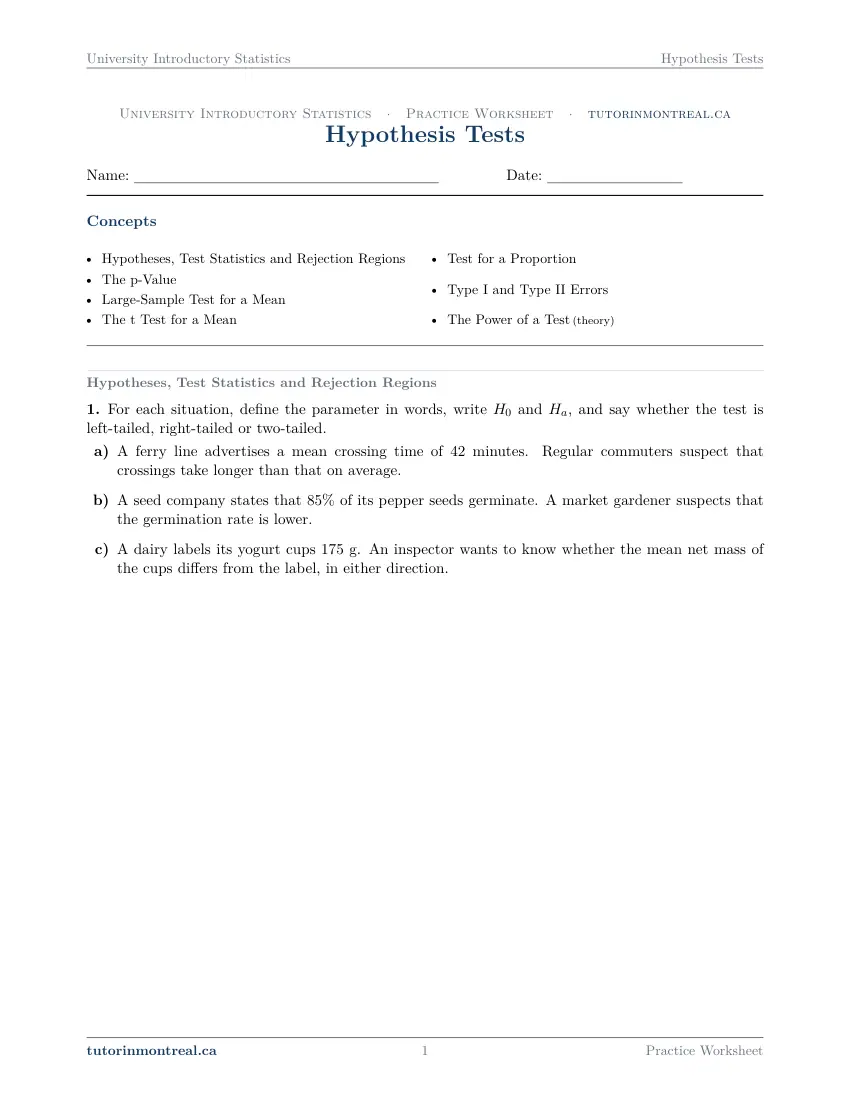
1. Q1Hypotheses, Test Statistics and Rejection Regions

   For each situation, define the parameter in words, write $H_0$ and $H_a$, and say whether the test is left-tailed, right-tailed or two-tailed.

   1. A ferry line advertises a mean crossing time of $42$ minutes. Regular commuters suspect that crossings take longer than that on average.
   2. A seed company states that $85\%$ of its pepper seeds germinate. A market gardener suspects that the germination rate is lower.
   3. A dairy labels its yogurt cups $175$~g. An inspector wants to know whether the mean net mass of the cups differs from the label, in either direction.
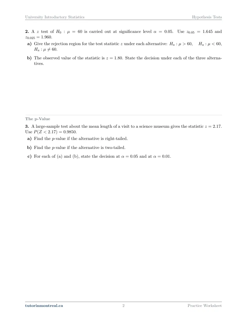
2. Q2Hypotheses, Test Statistics and Rejection Regions

   A $z$ test of $H_0:\mu =60$ is carried out at significance level $\alpha =0.05$. Use $z_{0.05}=1.645$ and $z_{0.025}=1.960$.

   1. Give the rejection region for the test statistic $z$ under each alternative: $H_a:\mu >60$, $H_a:\mu <60$, $H_a:\mu \ne 60$.
   2. The observed value of the statistic is $z=1.80$. State the decision under each of the three alternatives.
3. Q3The p-Value

   A large-sample test about the mean length of a visit to a science museum gives the statistic $z=2.17$. Use $P(Z<2.17)=0.9850$.

   1. Find the $p$-value if the alternative is right-tailed.
   2. Find the $p$-value if the alternative is two-tailed.
   3. For each of (a) and (b), state the decision at $\alpha =0.05$ and at $\alpha =0.01$.
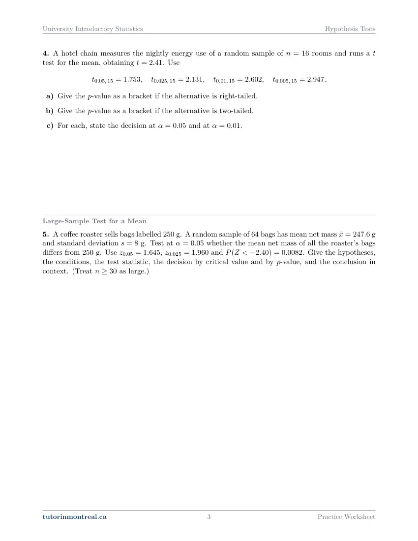
4. Q4The p-Value

   A hotel chain measures the nightly energy use of a random sample of $n=16$ rooms and runs a $t$ test for the mean, obtaining $t=2.41$. Use $$t_{0.05,15}=1.753,t_{0.025,15}=2.131,t_{0.01,15}=2.602,t_{0.005,15}=2.947.$$

   1. Give the $p$-value as a bracket if the alternative is right-tailed.
   2. Give the $p$-value as a bracket if the alternative is two-tailed.
   3. For each, state the decision at $\alpha =0.05$ and at $\alpha =0.01$.
5. Q5Large-Sample Test for a Mean

   A coffee roaster sells bags labelled $250$~g. A random sample of $64$ bags has mean net mass $\overline{x}=247.6$~g and standard deviation $s=8$~g. Test at $\alpha =0.05$ whether the mean net mass of all the roaster's bags differs from $250$~g. Use $z_{0.05}=1.645$, $z_{0.025}=1.960$ and $P(Z<-2.40)=0.0082$. Give the hypotheses, the conditions, the test statistic, the decision by critical value and by $p$-value, and the conclusion in context. (Treat $n\ge 30$ as large.)

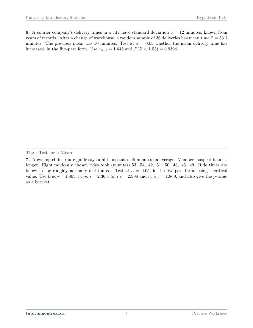
6. Q6Large-Sample Test for a Mean

   A courier company's delivery times in a city have standard deviation $\sigma =12$ minutes, known from years of records. After a change of warehouse, a random sample of $36$ deliveries has mean time $\overline{x}=53.1$ minutes. The previous mean was $50$ minutes. Test at $\alpha =0.05$ whether the mean delivery time has increased, in the five-part form. Use $z_{0.05}=1.645$ and $P(Z<1.55)=0.9394$.

7. Q7The t Test for a Mean

   A cycling club's route guide says a hill loop takes $45$ minutes on average. Members suspect it takes longer. Eight randomly chosen rides took (minutes) $53,54,42,51,50,48,45,49$. Ride times are known to be roughly normally distributed. Test at $\alpha =0.05$, in the five-part form, using a critical value. Use $t_{0.05,7}=1.895$, $t_{0.025,7}=2.365$, $t_{0.01,7}=2.998$ and $t_{0.05,8}=1.860$, and also give the $p$-value as a bracket.

8. Q8The t Test for a Mean

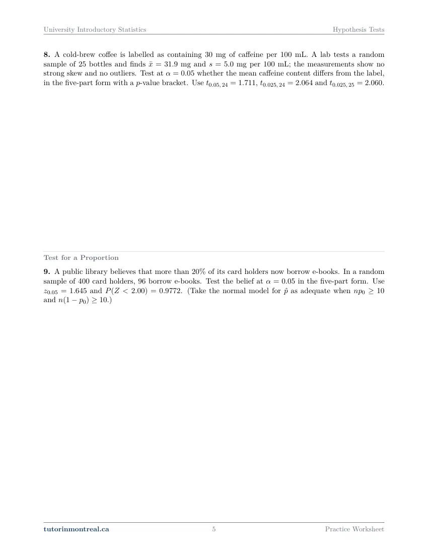
   A cold-brew coffee is labelled as containing $30$~mg of caffeine per $100$~mL. A lab tests a random sample of $25$ bottles and finds $\overline{x}=31.9$~mg and $s=5.0$~mg per $100$~mL; the measurements show no strong skew and no outliers. Test at $\alpha =0.05$ whether the mean caffeine content differs from the label, in the five-part form with a $p$-value bracket. Use $t_{0.05,24}=1.711$, $t_{0.025,24}=2.064$ and $t_{0.025,25}=2.060$.

9. Q9Test for a Proportion

   A public library believes that more than $20\%$ of its card holders now borrow e-books. In a random sample of $400$ card holders, $96$ borrow e-books. Test the belief at $\alpha =0.05$ in the five-part form. Use $z_{0.05}=1.645$ and $P(Z<2.00)=0.9772$. (Take the normal model for $\widehat{p}$ as adequate when $n{p}_0\ge 10$ and $n(1-p_0)\ge 10$.)

10. Q10Test for a Proportion

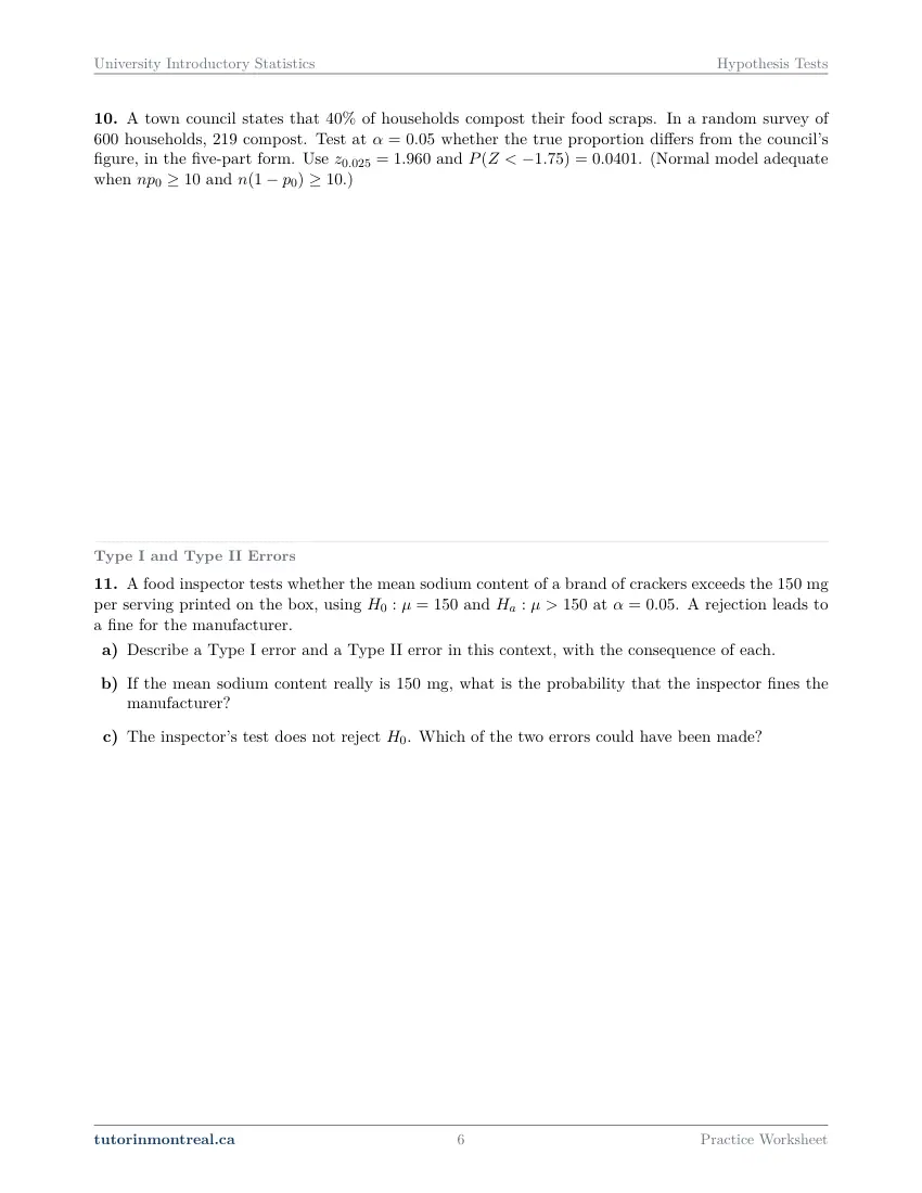
    A town council states that $40\%$ of households compost their food scraps. In a random survey of $600$ households, $219$ compost. Test at $\alpha =0.05$ whether the true proportion differs from the council's figure, in the five-part form. Use $z_{0.025}=1.960$ and $P(Z<-1.75)=0.0401$. (Normal model adequate when $n{p}_0\ge 10$ and $n(1-p_0)\ge 10$.)

11. Q11Type I and Type II Errors

    A food inspector tests whether the mean sodium content of a brand of crackers exceeds the $150$~mg per serving printed on the box, using $H_0:\mu =150$ and $H_a:\mu >150$ at $\alpha =0.05$. A rejection leads to a fine for the manufacturer.

    1. Describe a Type I error and a Type II error in this context, with the consequence of each.
    2. If the mean sodium content really is $150$~mg, what is the probability that the inspector fines the manufacturer?
    3. The inspector's test does not reject $H_0$. Which of the two errors could have been made?
12. Q12Type I and Type II Errors

    An electronics buyer receives fuses in large lots. From each lot it tests $10$ randomly chosen fuses and rejects the lot if $2$ or more are defective. Let $p$ be the proportion defective in a lot, with $H_0:p=0.05$ (an acceptable lot) and $H_a:p>0.05$, so that rejecting the lot is rejecting $H_0$. The number of defectives among the $10$ is binomial.

    1. Find the probability of a Type I error.
    2. Find the probability of a Type II error if in fact $p=0.20$.

    Give probabilities to four decimal places.

13. Q13The Power of a Test

    A decking manufacturer tests whether a new resin raises the mean breaking load of its boards above $500$~kg. It uses $H_0:\mu =500$, $H_a:\mu >500$ at $\alpha =0.05$, with a random sample of $64$ boards; the breaking loads have standard deviation $\sigma =40$~kg. Use $z_{0.05}=1.645$ and $P(Z<-0.755)=0.2251$.

    1. Find the values of $\overline{x}$ for which $H_0$ is rejected.
    2. Find the probability of a Type II error, and the power of the test, if the true mean breaking load is $512$~kg.
    3. Without further calculation, say whether the power at $\mu =512$ goes up or down if (i) $n$ is increased to $100$; (ii) $\alpha$ is lowered to $0.01$; (iii) the power is instead computed at $\mu =520$. Give a reason for each.
14. Q14Synthesis — drawing on several topics in this unit

    A water treatment plant must keep the mean dissolved-oxygen level of its outflow at $8.0$~mg/L or above. An inspector takes a random sample of $100$ readings and finds $\overline{x}=7.62$~mg/L and $s=1.9$~mg/L. The inspector tests $H_0:\mu =8.0$ against $H_a:\mu <8.0$. Use $P(Z<-2.00)=0.0228$.

    1. Check the conditions, compute the test statistic and the $p$-value.
    2. State the decision and the conclusion in context at $\alpha =0.01$, and then at $\alpha =0.05$.
    3. For each of the two decisions in (b), name the type of error that could have been made, and describe it in context.

The 10 challenge problems for this topic are a separate, paid sheet and are not reproduced here.

How to do every concept on this sheet

This is the part worksheet sites usually leave out. Below is the actual reasoning behind each group of questions — not a full solution set, the decisions that get you to one. Read it before you start, or after you get stuck.

Hypotheses, test statistics and rejection regions

A test never proves a claim. It asks whether the data are surprising under one specific assumption, and that assumption is H₀. Two rules fix the setup before any arithmetic: H₀ always states equality at a single value of the parameter, and Hₐ carries the direction that the question's own wording suspects — never a direction suggested by the sample after it has been looked at.

Q2 then separates the alternative from the arithmetic. The same value of z, tested at the same α, faces a different rejection region under each of the three alternatives, because the same total area is placed in one tail or split between two. Part (a) asks for the three regions in terms of the printed critical values, and part (b) applies one observed statistic to all three in turn. Write each region as an inequality in z before comparing anything, and say which printed critical value belongs to which region and why.

The p-value

A p-value answers a conditional question: if H₀ were true, how likely is a test statistic at least this extreme? It is an area in the tail — or tails — that Hₐ points to, measured from the observed statistic outward. It is not the probability that H₀ is true, and it is not the probability that the decision is wrong.

Q3 gives one z and one table value, P(Z < 2.17), and asks for the p-value under two different alternatives. The table reports area to the left, so a right-tailed p-value is one minus the printed figure; the two-tailed p-value doubles that one tail, because an equally extreme result on the other side would have counted too. Part (c) then compares the p-value with two different values of α. Do not compute a new statistic for the second α — the p-value is a property of the data and the alternative, and only the threshold it is compared against changes.

Q4 also asks for the decision at two levels of α, which is where a bracket earns its keep: when α falls outside the bracket the decision is settled, and when it falls inside it the bracket is too coarse and the honest answer says so. The decision rule itself is the same in every question on this sheet — reject H₀ when p ≤ α — and it agrees with the critical-value rule by construction, because both are asking whether the statistic has passed the same boundary.

The large-sample test for a mean

From here every question is asked in the same five-part form, and the form is the answer's structure, not a suggestion: hypotheses, conditions, test statistic, decision, conclusion in context.

The t test for a mean

When the sample is small and σ is unknown, s carries real uncertainty of its own, and the standardized statistic follows a t distribution rather than a normal one. The formula looks the same; the table it is compared against does not.

Q7 hands you eight raw ride times, so x̄ and s come first, from the data, before any test exists. The question states that ride times are roughly normally distributed — that is the condition being handed to you, and a small-sample t test needs it stated, so quote it in the conditions step rather than skipping past it. Q8 gives x̄ and s directly, and tells you instead that the measurements show no strong skew and no outliers, which is how the same condition is checked when the raw values are in hand.

Q7 asks for a decision by critical value and also for the p-value as a bracket, so the two routes appear side by side on the same test; Q8 is two-tailed, which means the printed critical value to compare against is the one carrying α/2 in each tail, and the bracket has to be doubled. Both close with a sentence about the loop or the caffeine content.

The test for a proportion

A proportion test is the same machine with a different standard error. The sample proportion is p̂ = x/n, and the standard error is built from the null value p₀ — not from p̂ — because the whole calculation is carried out under the assumption that H₀ is true.

Q9 and Q10 both print the size condition they want checked, np₀ ≥ 10 and n(1 − p₀) ≥ 10, and both give the counts rather than the proportion, so the first line of work is converting a count of card holders or of households into p̂. Q9's belief is one-sided and Q10's is two-sided, which is the only structural difference between them: one critical value is printed in each question, and it is the one that matches that question's tail.

Type I and Type II errors

Every test can be wrong in exactly two ways, and which one is available depends on the decision that was made. Rejecting a true H₀ is a Type I error; failing to reject a false H₀ is a Type II error. α is the probability of the first, fixed in advance by choosing the significance level; β is the probability of the second, and it is not fixed by anything until a specific alternative value of the parameter is named.

Q11(b) asks for a probability under the assumption that H₀ is exactly true; identify which of the two error probabilities that describes, and notice that the test has already fixed it rather than leaving it to be computed. Q11(c) is the pairing above, read backwards: a decision only risks the error that belongs to it, so settle which decision was taken before naming anything.

The power of a test

Power is the probability of rejecting H₀ when it is false by a specified amount: power = 1 − β. It cannot be computed from H₀ alone, because β is measured under a stated true value of μ, and that is why Q13 names one.

Q13(c) asks for directions only, with a reason for each, and forbids further calculation — so argue from the picture rather than from arithmetic. Each of the three changes moves either the cut-off or the curve the area is measured under: a larger n shrinks the standard error and so narrows both distributions; a smaller α pushes the cut-off further out; a more distant true mean slides the second curve away from the cut-off. Decide in each case which way the shaded region beyond the cut-off grows or shrinks, and write that as the reason.

The synthesis question

Q14 runs the whole sheet on one situation. Part (a) is the large-sample test for a mean with a one-sided alternative: check the conditions the sample size and the random draw give you, standardize with s in place of σ, and find the p-value from the supplied table value in the tail Hₐ points to. Part (b) then asks for the decision and the conclusion at two different values of α, and this is the point of the question — the data do not change and the statistic does not change; only the threshold moves. Compare the one p-value against each α in turn and let each comparison stand on its own, rather than carrying the first decision over to the second.

Part (c) closes the loop by attaching an error to each of those two decisions. Whichever way a decision goes, exactly one of the two errors is available to it, and describing it in context means naming what would be true of the outflow and what the inspector would have done about it. Each of the two decisions carries exactly one of the errors with it, which is the clearest argument in the set that α is chosen before the data are seen, not after.

Preview all 9 pages

Click any page to open the full PDF.

Getting the most out of it

Write the five parts as headings before you compute

Hypotheses, conditions, test statistic, decision, conclusion. Put the five labels down the page first and fill them in. Marks on these questions are attached to the parts, not to the final number, and the part most often missing is the conditions — which is also the part that decides whether z or t is legitimate at all.

Say the tail out loud before you open the table

One tail or two, and on which side. Nearly every wrong critical value and every wrong p-value on this sheet is that sentence skipped. Sketch the curve, shade the region Hₐ describes, and only then decide whether the table's left-tail area needs subtracting or doubling.

Finish in a sentence with no symbols in it

Every question here asks for a conclusion in context, and a conclusion that says "reject" and stops is unfinished. Name the population, the claim, the significance level, and whether the evidence was sufficient — in language the ferry line, the roaster or the town council would understand.

Keep α, the p-value and β apart in your head

α is chosen before the data and is the long-run rate of false rejections. The p-value is computed from the data and is an area measured from the observed statistic outward. β depends on a specific alternative value and cannot exist without one. Three different objects, all areas under a curve, and confusing any two of them produces an answer that looks reasonable and is not.

Check the two routes against each other

Where a question allows both, decide by critical value and by p-value and confirm they agree. They are the same comparison expressed in two scales, so a disagreement is a reliable signal that a tail was read wrongly — and it costs one extra line to find out.

Common questions