University Introductory Statistics — Two-Sample Inference and Chi-Square Tests Worksheet

11 of the 15 questions

Each question targets one named concept from the sheet. Read them here, or print the PDF — it has working space under each one. 11 of the 15 questions are printed below. The other 4 are built on a diagram or a table of values that does not translate to the page, so they are in the free PDF — marked below where they would have come.

1. Q1Large-Sample Inference for a Difference of Two Means

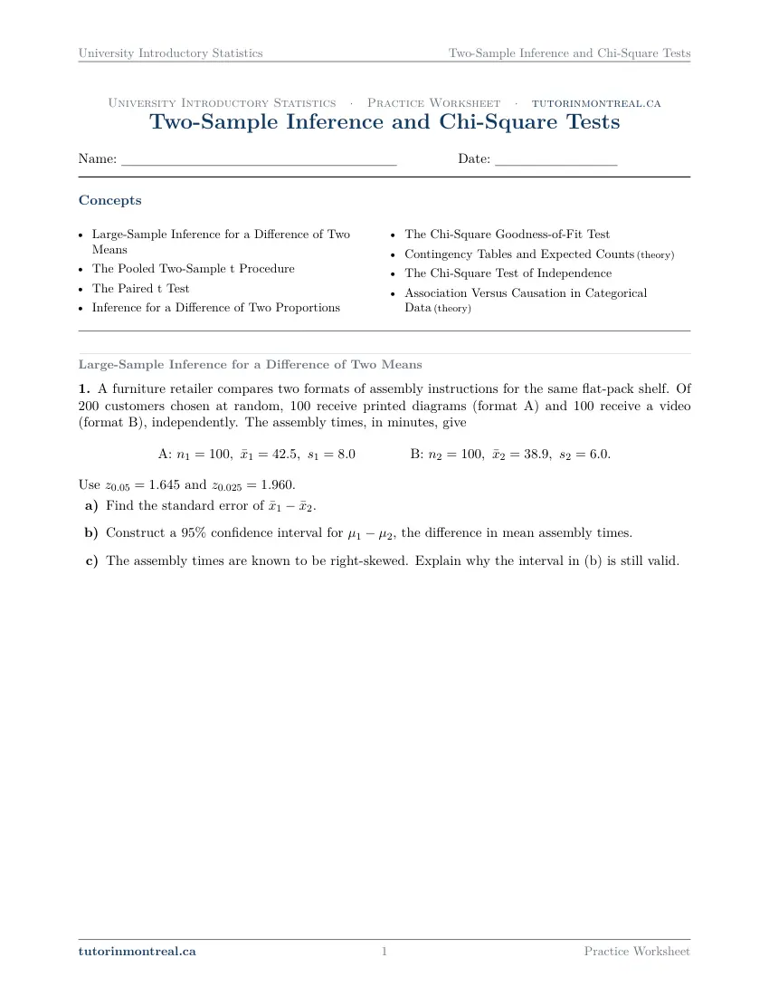
   A furniture retailer compares two formats of assembly instructions for the same flat-pack shelf. Of $200$ customers chosen at random, $100$ receive printed diagrams (format A) and $100$ receive a video (format B), independently. The assembly times, in minutes, give $$\text{A: }{n}_1=100,{\overline{x}}_1=42.5,s_1=8.0\text{B: }{n}_2=100,{\overline{x}}_2=38.9,s_2=6.0.$$ Use $z_{0.05}=1.645$ and $z_{0.025}=1.960$.

   1. Find the standard error of ${\overline{x}}_1-{\overline{x}}_2$.
   2. Construct a $95\%$ confidence interval for ${\mu }_1-{\mu }_2$, the difference in mean assembly times.
   3. The assembly times are known to be right-skewed. Explain why the interval in (b) is still valid.
2. Q2Large-Sample Inference for a Difference of Two Means

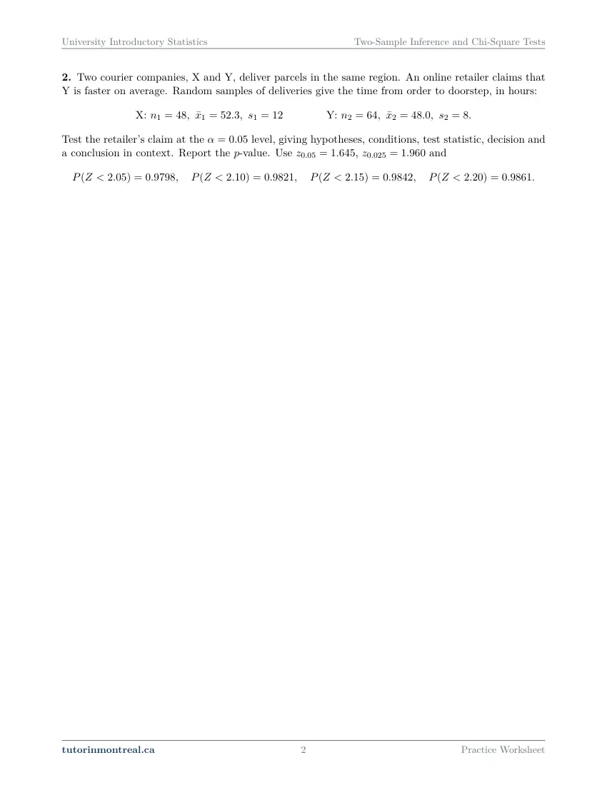
   Two courier companies, X and Y, deliver parcels in the same region. An online retailer claims that Y is faster on average. Random samples of deliveries give the time from order to doorstep, in hours: $$\text{X: }{n}_1=48,{\overline{x}}_1=52.3,s_1=12\text{Y: }{n}_2=64,{\overline{x}}_2=48.0,s_2=8.$$ Test the retailer's claim at the $\alpha =0.05$ level, giving hypotheses, conditions, test statistic, decision and a conclusion in context. Report the $p$-value. Use $z_{0.05}=1.645$, $z_{0.025}=1.960$ and $$P(Z<2.05)=0.9798,P(Z<2.10)=0.9821,P(Z<2.15)=0.9842,P(Z<2.20)=0.9861.$$

3. Q3The Pooled Two-Sample t Procedure

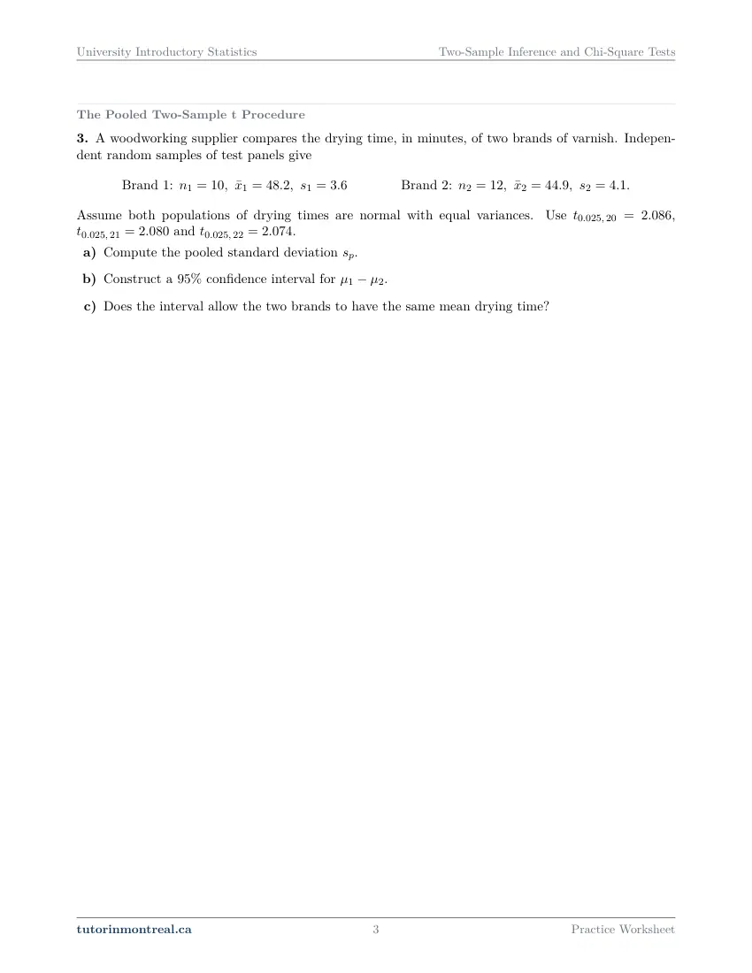
   A woodworking supplier compares the drying time, in minutes, of two brands of varnish. Independent random samples of test panels give $$\text{Brand 1: }{n}_1=10,{\overline{x}}_1=48.2,s_1=3.6\text{Brand 2: }{n}_2=12,{\overline{x}}_2=44.9,s_2=4.1.$$ Assume both populations of drying times are normal with equal variances. Use $t_{0.025,20}=2.086$, $t_{0.025,21}=2.080$ and $t_{0.025,22}=2.074$.

   1. Compute the pooled standard deviation $s_p$.
   2. Construct a $95\%$ confidence interval for ${\mu }_1-{\mu }_2$.
   3. Does the interval allow the two brands to have the same mean drying time?
4. Q4The Pooled Two-Sample t Procedure

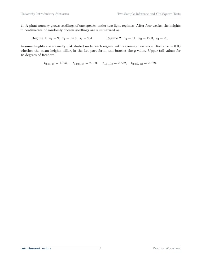
   A plant nursery grows seedlings of one species under two light regimes. After four weeks, the heights in centimetres of randomly chosen seedlings are summarized as $$\text{Regime 1: }{n}_1=9,{\overline{x}}_1=14.6,s_1=2.4\text{Regime 2: }{n}_2=11,{\overline{x}}_2=12.3,s_2=2.0.$$ Assume heights are normally distributed under each regime with a common variance. Test at $\alpha =0.05$ whether the mean heights differ, in the five-part form, and bracket the $p$-value. Upper-tail values for $18$ degrees of freedom: $$t_{0.05,18}=1.734,t_{0.025,18}=2.101,t_{0.01,18}=2.552,t_{0.005,18}=2.878.$$

5. Q5The Paired t Test

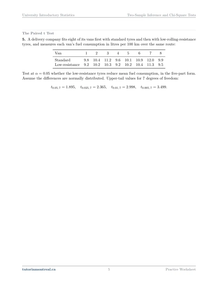
   This question is built around a diagram or a table of values. Open it in the PDF.

6. Q6The Paired t Test

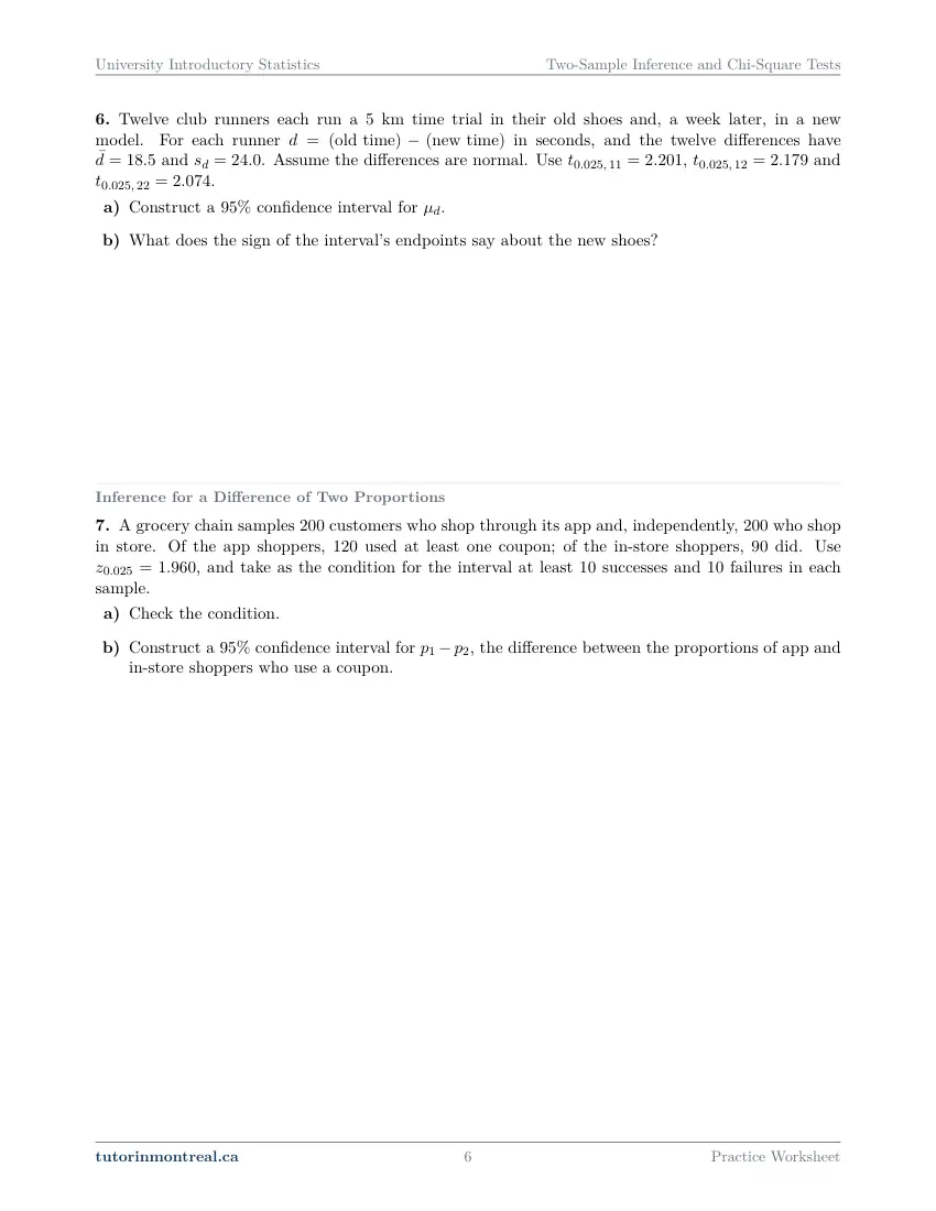
   Twelve club runners each run a $5$ km time trial in their old shoes and, a week later, in a new model. For each runner $d=(\text{old time})-(\text{new time})$ in seconds, and the twelve differences have $\overline{d}=18.5$ and $s_d=24.0$. Assume the differences are normal. Use $t_{0.025,11}=2.201$, $t_{0.025,12}=2.179$ and $t_{0.025,22}=2.074$.

   1. Construct a $95\%$ confidence interval for ${\mu }_d$.
   2. What does the sign of the interval's endpoints say about the new shoes?
7. Q7Inference for a Difference of Two Proportions

   A grocery chain samples $200$ customers who shop through its app and, independently, $200$ who shop in store. Of the app shoppers, $120$ used at least one coupon; of the in-store shoppers, $90$ did. Use $z_{0.025}=1.960$, and take as the condition for the interval at least $10$ successes and $10$ failures in each sample.

   1. Check the condition.
   2. Construct a $95\%$ confidence interval for $p_1-p_2$, the difference between the proportions of app and in-store shoppers who use a coupon.
8. Q8Inference for a Difference of Two Proportions

   A dental clinic compares two appointment reminders. Of $160$ patients chosen at random to receive a text message, $48$ missed their appointment; of $150$ patients chosen at random to receive a phone call, $30$ missed theirs. Test at $\alpha =0.05$ whether the no-show rates differ, in the five-part form, and give the $p$-value. Take as the condition at least $10$ expected successes and failures in each sample under $H_0$. Use $z_{0.025}=1.960$ and $$P(Z<2.00)=0.9772,P(Z<2.03)=0.9788,P(Z<2.05)=0.9798.$$

9. Q9The Chi-Square Goodness-of-Fit Test

   A municipal helpline wants to know whether calls are spread evenly across the five weekdays. In a random sample of $200$ calls, the counts from Monday to Friday are $32,38,41,47,42$. Test at $\alpha =0.05$ whether the calls are uniformly distributed over the weekdays, in the five-part form; the test requires every expected count to be at least $5$. Use ${\chi }_{0.10,4}^2=7.779$, ${\chi }_{0.05,4}^2=9.488$ and ${\chi }_{0.05,5}^2=11.070$.

10. Q10The Chi-Square Goodness-of-Fit Test

    A ferry operator's planning assumes that its passengers are $60\%$ foot passengers, $25\%$ travelling with a car and $15\%$ with a bicycle. A random sample of $160$ passengers contains $80$ on foot, $52$ with a car and $28$ with a bicycle. Test the assumption at $\alpha =0.05$ in the five-part form and bracket the $p$-value. The test requires every expected count to be at least $5$. Upper-tail values: $${\chi }_{0.05,2}^2=5.991,{\chi }_{0.025,2}^2=7.378,{\chi }_{0.01,2}^2=9.210,{\chi }_{0.05,3}^2=7.815.$$

11. Q11Contingency Tables and Expected Counts

    This question is built around a diagram or a table of values. Open it in the PDF.

12. Q12The Chi-Square Test of Independence

    This question is built around a diagram or a table of values. Open it in the PDF.

13. Q13The Chi-Square Test of Independence

    This question is built around a diagram or a table of values. Open it in the PDF.

14. Q14Association Versus Causation in Categorical Data

    A random sample of households in one city is classified by whether the home has a smoke detector that works and whether the household reported a kitchen fire in the past five years. A chi-square test of independence gives $p=0.002$. For each statement, say whether the study supports it, and give a one-line reason.

    1. Having a working smoke detector and reporting a kitchen fire are associated in this city's households.
    2. Installing a working smoke detector changes a household's chance of a kitchen fire.
    3. If the two variables were independent, a table at least this far from the expected counts would occur in about $0.2\%$ of samples.
    4. The result applies to households in every city.
15. Q15Synthesis — drawing on several topics in this unit

    A library tests two wordings of an overdue-book email. Of $120$ borrowers chosen at random to receive wording 1, $45$ return the book within a week; of $120$ receiving wording 2, $30$ do. The $z$ test requires at least $10$ expected successes and $10$ expected failures in each group under $H_0$, and the chi-square test every expected count at least $5$. Use ${\chi }_{0.05,1}^2=3.841$, $z_{0.025}=1.960$ and $P(Z<2.09)=0.9817$.

    1. Carry out the two-sided pooled $z$ test of $H_0:p_1=p_2$ and give its $p$-value.
    2. Arrange the data as a $2\times 2$ table and compute the chi-square statistic for independence of wording and prompt return.
    3. Compare $z^2$ with ${\chi }^2$, and compare the two decisions at $\alpha =0.05$.

The 9 challenge problems for this topic are a separate, paid sheet and are not reproduced here.

How to do every concept on this sheet

This is the part worksheet sites usually leave out. Below is the actual reasoning behind each group of questions — not a full solution set, the decisions that get you to one. Read it before you start, or after you get stuck.

Large-sample inference for a difference of two means

Everything in this set is one estimate minus another, and the first job is always the same: find the standard error of the difference. Two independent samples have independent means, so the variances add — never the standard deviations.

Q1(a) asks for exactly that quantity, and Q1(b) wraps it in the usual interval, (x̄₁ − x̄₂) ± z × SE. Two critical values are printed in Q1; only one of them belongs to a two-sided interval at the confidence level asked for, and choosing between them is part of the question. Keep the subtraction in the order the question defines — the wording fixes which population is 1 and which is 2, and reversing it reverses the sign of both endpoints and the meaning of the sentence you write about them.

This procedure replaces each unknown population standard deviation by its sample value and still uses a z critical value, which is only safe when both samples are large — so that condition goes on the page before the arithmetic, not after it. Q1(c) is the part that carries the marks: it tells you the populations are skewed and asks why the interval is still usable. The justification is not about the data being normal — it is a statement about the sampling distribution of a mean, and it has a condition attached. Name the result, say what it does to each sample mean, and say what it needs.

Q2 is the same machinery as a test. The retailer's claim points in one direction, so the alternative hypothesis is one-sided and the p-value comes from one tail only. Write H₀ as an equality between the two population means (or, equivalently, μ₁ − μ₂ = 0), and put the claim in the alternative — a claim is what you are trying to find evidence for, never what you assume. Four normal-table values are printed; the one you need is the one nearest your test statistic, and reading the p-value off the wrong tail is the standard way to lose the question after doing the arithmetic correctly.

The pooled two-sample t procedure

When both samples are small, the sample standard deviations are too unreliable to be treated as if they were the population values, and the z procedure is replaced by a t one. The version used throughout this set assumes a common population variance, which the question states for you, and estimates it by a weighted average of the two sample variances.

Q3(a) asks for sₚ itself. Note the shape of the weights: the larger sample pulls the pooled value towards its own standard deviation, and sₚ always lands between s₁ and s₂ — a free check on the arithmetic before you go any further. Q3(b) builds the interval with that SE and a t critical value.

Q3(c) asks whether the interval leaves room for the two means to be equal. The rule is general and worth stating in your own words before you use it: an interval for a difference is a set of plausible values for μ₁ − μ₂, so equality is plausible exactly when 0 is one of the values in the interval. Answer by saying where 0 sits relative to your two endpoints, not by comparing x̄₁ with x̄₂.

Q4 runs the same procedure as a test, in the five-part form, with a two-sided alternative because "differ" names no direction. Four upper-tail t values at the right degrees of freedom are printed so that the p-value can be bracketed: find the two printed values your statistic falls between and report the corresponding range. With a two-sided alternative the tail areas are doubled, and forgetting to double them is what turns a correct statistic into a wrong bracket. A bracket is a complete answer here — a printed table cannot give more.

Paired data, and why the design decides the test

Q5 and Q6 look like two-sample problems and are not. In both, the two measurements belong to the same unit — the same van, the same runner — so the two columns are not independent samples and the two-sample standard error does not apply. Reduce each pair to a single difference and run a one-sample t procedure on those differences.

Q5 asks whether one treatment reduces the mean, so the alternative is one-sided and the tail values printed for it are upper-tail values at the paired degrees of freedom. Q6 asks instead for an interval for the mean difference and then, in part (b), for what the signs of the two endpoints say about the new shoes. Three readings are possible — both endpoints on the same side of 0, or 0 between them — and each means something different about the direction of the change. Say which of the three you are in and what it implies, in the units the question uses.

A difference of two proportions

Each group supplies a sample proportion p̂ = (count)/(sample size), and the two are compared the same way two means were. What is new is that the interval and the test use different standard errors, and knowing why is the point of Q7 and Q8.

Q7(a) asks you to check the size condition the question states, and it has to be checked in all four places: successes and failures, in each of the two samples. Then Q7(b) is the interval in the usual shape, (p̂₁ − p̂₂) ± z × SE, with the subtraction in the order the question names.

Q8 is the two-sided test in the five-part form. Two things to keep straight: the "success" here is the event the counts are counting, so define it explicitly before writing any p̂, and the condition is stated in terms of expected counts under H₀ — that is, using the pooled proportion, not the separate ones. The p-value is two-sided, so the printed normal-table values give one tail only and the area on the far side has to be accounted for as well.

The chi-square goodness-of-fit test

Now the data are counts in categories rather than measurements, and the question is whether one set of counts is consistent with a stated model. The statistic measures the total relative discrepancy between what was observed and what the model predicts.

Q9's model is the uniform one — "spread evenly" means every category has the same probability, so each expected count is the sample size divided by the number of categories. Q10's model states unequal percentages, so each expected count is the sample size times that category's stated proportion. In both, the expected counts need not be whole numbers, and rounding them to integers before squaring is a real source of error. A quick check before continuing: the expected counts must add to the sample size.

Q10 also asks for a bracketed p-value, from the three upper-tail values printed at its degrees of freedom. Find the two your statistic falls between and report the interval between the corresponding tail areas; if it falls beyond the largest printed value, the p-value is smaller than that value's area, and saying so is the complete answer. Both questions state the expected-count condition — every expected count at least 5 — and both expect it verified against the counts you computed, not asserted.

Contingency tables and expected counts

Q11 does the arithmetic that the test of independence rests on, and does it on its own so that the next two questions can be about the test rather than about the table. Under the hypothesis that the row variable and the column variable are independent, the probability of a cell is the product of its row and column probabilities, and multiplying that by the grand total collapses to one formula.

Q11(a) asks for every cell. Work across a row at a time and use the margins as a running check: the expected counts in any row must add to that row's observed total, and the same for every column. That check catches a transposed pair of totals immediately, which no later step will. Q11(b) then asks for the expected-count condition and for the degrees of freedom of the test of independence, which come from the shape of the table alone. Count only the rows and columns of the data: the "Total" row and the "Total" column printed in the table are margins, not categories, and including them is the commonest way this number comes out wrong.

The chi-square test of independence

Q12 and Q13 put Q11's expected counts into Q9's statistic. The hypotheses are now statements about two categorical variables: H₀ says they are independent in the population sampled, and the alternative says only that they are not — there is no direction and no one-sided version of this test.

Q12 asks for the statistic, its degrees of freedom and a decision at the stated level. Set the work out as one row per cell — observed, expected, O − E, (O − E)²/E — and add the last column. Every term is non-negative, so a negative total means a sign was kept where it should have been squared away. Two of the three printed critical values sit at the degrees of freedom the table actually has and one does not; pick by computing df, not by eye.

Q13 is the larger table, in the five-part form, with a bracketed p-value from the printed upper-tail values. The conditions to write down are the random sampling the question describes and the expected-count rule, checked cell by cell on the expected counts you computed. The conclusion sentence has to name both variables in context — study location and programme — because "the variables are associated" is a sentence about symbols, not about students.

What a small p-value does and does not license

Q14 is the interpretation question the whole set has been building towards, and it is worth as much as any computation. A chi-square test on an observational sample has been run and its p-value is given; four statements are offered, and each has to be judged and justified in a line. Three distinctions decide all four.

The synthesis question

Q15 analyses one set of data twice. Part (a) is Q8's procedure: define the success, pool the two counts under H₀, and run the two-sided z test with the printed normal-table value. Part (b) takes the same four counts, arranges them as a two-by-two table — the two wordings as rows, the two outcomes as columns, with the margins you compute from them — and runs Q11's expected-count formula into Q12's statistic.

Part (c) then asks you to square the z from part (a), set it beside the χ² from part (b), and compare the two decisions at the stated level. Keep several decimal places through both parts rather than rounding at each step — a relationship between two quantities is invisible if rounding has already moved them apart. Each condition the question states belongs to one of the two procedures, so check them separately rather than assuming the second inherits the first.

Preview all 13 pages

Click any page to open the full PDF.

Getting the most out of it

Name the design before you reach for a formula

Three questions, in this order, and they settle everything: are the data measurements or counts in categories? If measurements, are the two groups independent or is each observation paired with another? If independent, are the samples large enough for z or small enough to need the pooled t? Almost every lost mark in this chapter is a correct procedure applied to the wrong design, and no amount of careful arithmetic afterwards recovers it.

Write the standard error on its own line

Every interval in this set is estimate ± critical value × SE and every test statistic is (estimate − hypothesised value)/SE. Computing the SE separately, labelled, before assembling anything means one quantity to check rather than a whole expression, and it makes the interval and the test share the work instead of repeating it.

Get the degrees of freedom from a formula, never from the printed list

n₁ + n₂ − 2 for the pooled t, n − 1 pairs for the paired t, k − 1 for goodness of fit, (r − 1)(c − 1) for independence. The questions print neighbouring critical values on purpose. Compute the number first and then find it; choosing the value that looks familiar is the error those neighbours are there to catch.

Check conditions in writing, before the arithmetic

Randomisation and independence, the sample sizes or the stated normality, the successes and failures in each group, every expected count against its floor. These carry marks in their own right in the five-part form, and a condition that fails changes what you are allowed to conclude — which is not something to discover after the test statistic is on the page.

Finish every question with a sentence about the subject

Vans, seedlings, no-show rates, weekdays, commuting modes. A decision about H₀ is an intermediate result; the answer is what it means for the two groups being compared, said in the units of the problem, with the uncertainty still attached. Every outline for this course asks for interpretation beside computation, and a question that ends at a number is unfinished.

Common questions