University Introductory Statistics — Sampling Distributions and the Central Limit Theorem Worksheet

All 9 questions

Each question targets one named concept from the sheet. Read them here, or print the PDF — it has working space under each one.

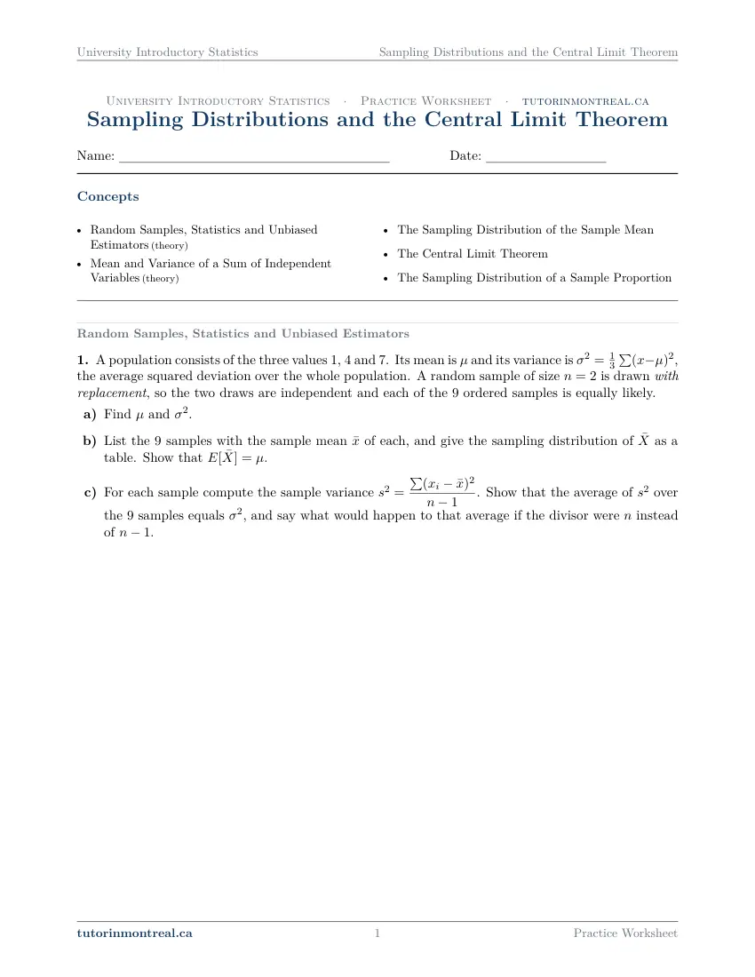
1. Q1Random Samples, Statistics and Unbiased Estimators

   A population consists of the three values $1$, $4$ and $7$. Its mean is $\mu$ and its variance is ${\sigma }^2=\frac{1}{3}\sum (x-\mu {)}^2$, the average squared deviation over the whole population. A random sample of size $n=2$ is drawn with replacement, so the two draws are independent and each of the $9$ ordered samples is equally likely.

   1. Find $\mu$ and ${\sigma }^2$.
   2. List the $9$ samples with the sample mean $\overline{x}$ of each, and give the sampling distribution of $\overline{X}$ as a table. Show that $E[\overline{X}]=\mu$.
   3. For each sample compute the sample variance $s^2={\displaystyle \frac{\sum (x_i-\overline{x}{)}^2}{n-1}}$. Show that the average of $s^2$ over the $9$ samples equals ${\sigma }^2$, and say what would happen to that average if the divisor were $n$ instead of $n-1$.
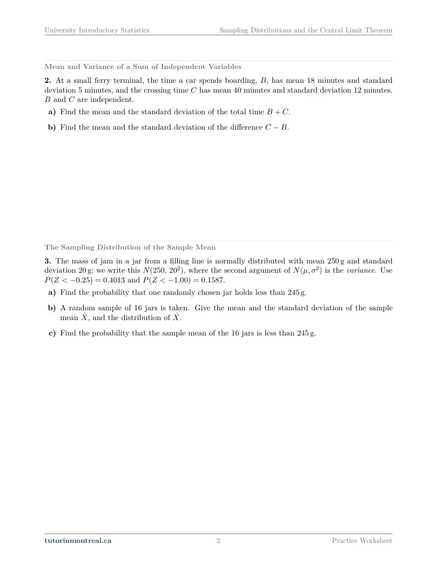
2. Q2Mean and Variance of a Sum of Independent Variables

   At a small ferry terminal, the time a car spends boarding, $B$, has mean $18$ minutes and standard deviation $5$ minutes, and the crossing time $C$ has mean $40$ minutes and standard deviation $12$ minutes. $B$ and $C$ are independent.

   1. Find the mean and the standard deviation of the total time $B+C$.
   2. Find the mean and the standard deviation of the difference $C-B$.
3. Q3The Sampling Distribution of the Sample Mean

   The mass of jam in a jar from a filling line is normally distributed with mean $250$ g and standard deviation $20$ g; we write this $N(250,{20}^2)$, where the second argument of $N(\mu ,{\sigma }^2)$ is the variance. Use $P(Z<-0.25)=0.4013$ and $P(Z<-1.00)=0.1587$.

   1. Find the probability that one randomly chosen jar holds less than $245$ g.
   2. A random sample of $16$ jars is taken. Give the mean and the standard deviation of the sample mean $\overline{X}$, and the distribution of $\overline{X}$.
   3. Find the probability that the sample mean of the $16$ jars is less than $245$ g.
4. Q4The Sampling Distribution of the Sample Mean

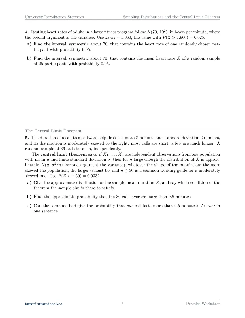
   Resting heart rates of adults in a large fitness program follow $N(70,{10}^2)$, in beats per minute, where the second argument is the variance. Use $z_{0.025}=1.960$, the value with $P(Z>1.960)=0.025$.

   1. Find the interval, symmetric about $70$, that contains the heart rate of one randomly chosen participant with probability $0.95$.
   2. Find the interval, symmetric about $70$, that contains the mean heart rate $\overline{X}$ of a random sample of $25$ participants with probability $0.95$.
5. Q5The Central Limit Theorem

   The duration of a call to a software help desk has mean $8$ minutes and standard deviation $6$ minutes, and its distribution is moderately skewed to the right: most calls are short, a few are much longer. A random sample of $36$ calls is taken, independently.

   The central limit theorem says: if $X_1,\dots ,X_n$ are independent observations from one population with mean $\mu$ and finite standard deviation $\sigma$, then for $n$ large enough the distribution of $\overline{X}$ is approximately $N(\mu ,{\sigma }^2/n)$ (second argument the variance), whatever the shape of the population; the more skewed the population, the larger $n$ must be, and $n\ge 30$ is a common working guide for a moderately skewed one. Use $P(Z<1.50)=0.9332$.

   1. Give the approximate distribution of the sample mean duration $\overline{X}$, and say which condition of the theorem the sample size is there to satisfy.
   2. Find the approximate probability that the $36$ calls average more than $9.5$ minutes.
   3. Can the same method give the probability that one call lasts more than $9.5$ minutes? Answer in one sentence.
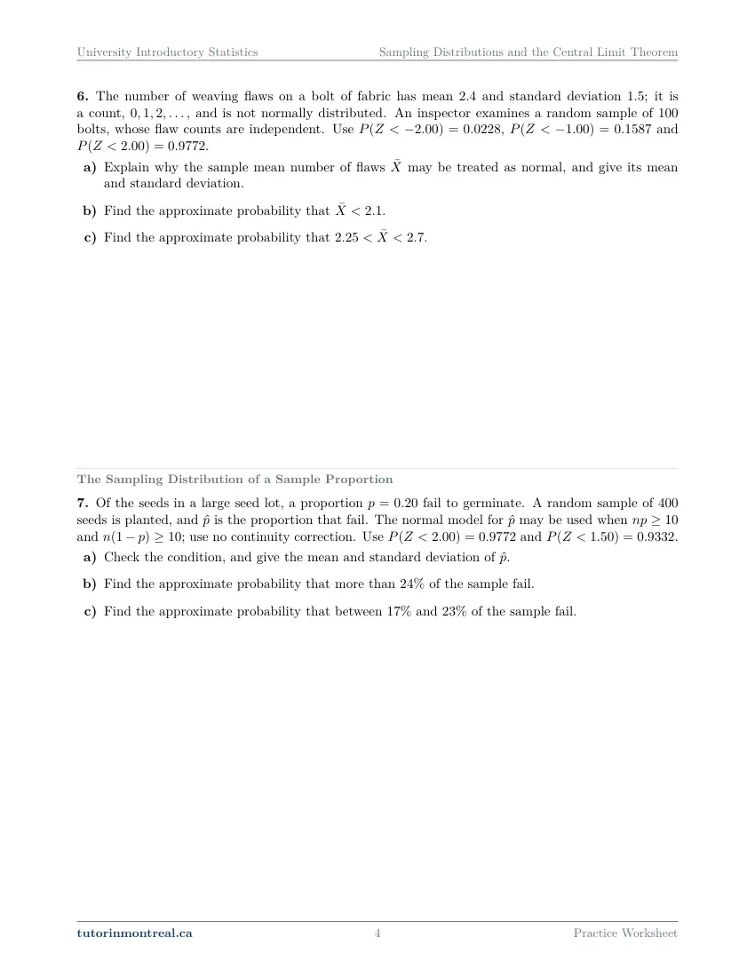
6. Q6The Central Limit Theorem

   The number of weaving flaws on a bolt of fabric has mean $2.4$ and standard deviation $1.5$; it is a count, $0,1,2,\dots$, and is not normally distributed. An inspector examines a random sample of $100$ bolts, whose flaw counts are independent. Use $P(Z<-2.00)=0.0228$, $P(Z<-1.00)=0.1587$ and $P(Z<2.00)=0.9772$.

   1. Explain why the sample mean number of flaws $\overline{X}$ may be treated as normal, and give its mean and standard deviation.
   2. Find the approximate probability that $\overline{X}<2.1$.
   3. Find the approximate probability that $2.25<\overline{X}<2.7$.
7. Q7The Sampling Distribution of a Sample Proportion

   Of the seeds in a large seed lot, a proportion $p=0.20$ fail to germinate. A random sample of $400$ seeds is planted, and $\widehat{p}$ is the proportion that fail. The normal model for $\widehat{p}$ may be used when $np\ge 10$ and $n(1-p)\ge 10$; use no continuity correction. Use $P(Z<2.00)=0.9772$ and $P(Z<1.50)=0.9332$.

   1. Check the condition, and give the mean and standard deviation of $\widehat{p}$.
   2. Find the approximate probability that more than $24\%$ of the sample fail.
   3. Find the approximate probability that between $17\%$ and $23\%$ of the sample fail.
8. Q8The Sampling Distribution of a Sample Proportion

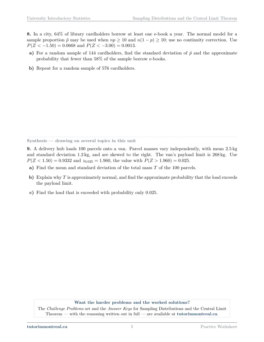
   In a city, $64\%$ of library cardholders borrow at least one e-book a year. The normal model for a sample proportion $\widehat{p}$ may be used when $np\ge 10$ and $n(1-p)\ge 10$; use no continuity correction. Use $P(Z<-1.50)=0.0668$ and $P(Z<-3.00)=0.0013$.

   1. For a random sample of $144$ cardholders, find the standard deviation of $\widehat{p}$ and the approximate probability that fewer than $58\%$ of the sample borrow e-books.
   2. Repeat for a random sample of $576$ cardholders.
9. Q9Synthesis — drawing on several topics in this unit

   A delivery hub loads $100$ parcels onto a van. Parcel masses vary independently, with mean $2.5$ kg and standard deviation $1.2$ kg, and are skewed to the right. The van's payload limit is $268$ kg. Use $P(Z<1.50)=0.9332$ and $z_{0.025}=1.960$, the value with $P(Z>1.960)=0.025$.

   1. Find the mean and standard deviation of the total mass $T$ of the $100$ parcels.
   2. Explain why $T$ is approximately normal, and find the approximate probability that the load exceeds the payload limit.
   3. Find the load that is exceeded with probability only $0.025$.

The 7 challenge problems for this topic are a separate, paid sheet and are not reproduced here.

How to do every concept on this sheet

This is the part worksheet sites usually leave out. Below is the actual reasoning behind each group of questions — not a full solution set, the decisions that get you to one. Read it before you start, or after you get stuck.

Random samples, statistics and unbiased estimators

A statistic — x̄, s², p̂ — is computed from a sample, and a different sample would have given a different value. That is the whole idea of the chapter: the statistic is itself a random variable, and it has a distribution of its own, called its sampling distribution. Q1 builds one from nothing, on a population small enough to write out in full.

Q1(a) asks for the population mean and the population variance first, and the formula printed in the question is the population one: the squared deviations are averaged over all three values, with no n − 1 anywhere. Keep that number to one side; it is the target that Q1(b) and Q1(c) compare against.

The mean and variance of a sum of independent variables

Q2 is the small piece of algebra that every standard error in the rest of the course is built from. Two rules, and the difference between them is where marks are lost.

Q2(b) changes the sign in the mean but not in the variance. Subtracting a variable does not remove uncertainty — the crossing time and the boarding time are each uncertain, and their difference inherits both uncertainties — so the plus sign in the variance rule stands whichever way the means go. Write the variance line out before touching Q2(b) and the sign takes care of itself.

The sampling distribution of the sample mean

When the population itself is normal, no approximation is needed: x̄ is exactly normal, centred at the same place as the population, and narrower by a factor of √n.

Q3 states its distribution as N(250, 20²) and tells you that the second argument is the variance — read that convention carefully, because a distribution written with a variance inside and a standard deviation wanted outside is where a factor of a square root goes astray. Q3(a) is a single jar, so the spread is σ. Q3(b) asks for the mean, the standard deviation and the distribution of x̄ for a sample of 16; name the distribution in full, not just its two numbers. Q3(c) is the same threshold as Q3(a) asked of the sample mean instead.

Q4 runs the standardizing backwards. A central interval with probability 0.95 is built by starting from the value z = 1.960 that the question supplies and undoing the standardizing — μ ± z × (the spread of whatever is being measured). Q4(a) is one participant, so the spread is σ; Q4(b) is the mean of 25, so the spread is σ/√25. Symmetric about the mean means the two endpoints are the same distance either side, so one multiplication does the whole job.

The central limit theorem

Q3 and Q4 had a normal population to start from. The central limit theorem is what to do when there is not one. Its statement is printed in Q5, and it is worth reading as a list of conditions rather than as a sentence: independent observations, one population, a finite standard deviation, and n large enough for the shape of that population.

Q5(a) asks not only for the distribution but for which condition of the theorem the sample size is there to satisfy — quote the condition from the statement in the question and match it to the skew described in the first paragraph. Q5(b) is step 4. Q5(c) asks whether the same method reaches one single call, and it is answered by asking what the theorem is a statement about: it describes the behaviour of x̄, and it says nothing about the shape of the population itself. One sentence, naming what you would have to know about that shape to work with a single call.

Q6 puts the theorem on a count, which is as far from normal as this set goes: the number of flaws cannot be negative, can only be a whole number, and has a standard deviation not much smaller than its mean. Q6(a) asks you to explain, so write the conditions out and say which feature of the sample makes each one hold, then give the two numbers for x̄. Q6(b) is a one-sided probability; Q6(c) is a between, which is the difference of two table readings — standardize each endpoint, and subtract the smaller cumulative value from the larger. Sketching the curve and shading the strip before subtracting is what keeps that subtraction the right way round.

The sampling distribution of a sample proportion

A proportion is a mean in disguise — the mean of a variable that is 1 when the thing happens and 0 when it does not — so p̂ gets a sampling distribution by the same argument, with its own formula for the spread.

Q7(a) asks for the condition to be checked, not assumed: compute both np and n(1 − p) and write them down beside the requirement. It is a condition on two quantities, not one, because a proportion close to 0 or to 1 needs a much larger sample before the normal shape is any good. Both Q7 and Q8 state that no continuity correction is to be used, so the calculation is the plain standardizing of Q3 with √(p(1 − p)/n) in place of σ/√n.

Q8 asks the same question of two sample sizes, and the comparison is the point of the question. Only n moves between Q8(a) and Q8(b); p, and therefore p(1 − p), is the same in both. Because n sits under a square root, multiplying the sample size by four divides the standard deviation of p̂ by two, and the same distance from p is then worth twice as many standard deviations. Set the two z-scores of Q8(a) and Q8(b) side by side before reading either from the table.

The synthesis question

Q9 uses a total rather than an average, and the sheet has already supplied the rule: a total of n independent observations is the sum of Q2, repeated n times.

Note the two different powers of n in Q9(a) — the mean is multiplied by n, the standard deviation only by √n — which is the same fact as SD(x̄) = σ/√n seen from the other side. Q9(b) is Q5 and Q6's explanation, applied to a sum: the central limit theorem covers a total as readily as an average, since one is a fixed multiple of the other, and the skew of the individual parcel masses is what makes the sample size worth remarking on. Then standardize the payload limit against the mean and standard deviation from Q9(a).

Q9(c) runs it backwards, like Q4: you are given a probability and asked for the value, so start from the supplied z and write value = mean + z × standard deviation, with the mean and standard deviation of the total rather than of one parcel. Decide from the wording which side of the centre the answer must fall on, and check your result against that expectation before writing it down.

Preview all 5 pages

Click any page to open the full PDF.

Getting the most out of it

Name the distribution before every calculation

One observation, a sample mean, a sample proportion, a total: four different spreads, one shared table. Write the distribution and its two parameters on their own line before any standardizing, and most of the errors in this chapter never get the chance to happen.

Divide by √n, never by n

The variance of x̄ carries n; the standard deviation carries √n. Decide which of the two the question wrote down — Q3 and Q5 both state a distribution with the variance inside — and convert once, deliberately, rather than at the moment of substituting.

Check conditions in writing, not in your head

Independence, a finite standard deviation, a sample size against the guide for a skewed population, np ≥ 10 and n(1 − p) ≥ 10. Q6(a) and Q7(a) award marks for the check itself, and every later chapter of this course opens with one.

Sketch the curve and shade before you subtract

A between-probability, such as Q6(c) or Q7(c), is one table value minus another, and the order is decided by the picture. Thirty seconds of sketching is cheaper than a negative probability.

Read every number the question hands you

These sheets print the table values you will need and nothing else. If a z you computed matches none of them, stop: the denominator, the conversion from per cent, or the choice between σ and σ/√n has gone wrong, and the supplied list has told you so before the answer did.

Common questions