University Introductory Statistics — Simple Linear Regression and Correlation Worksheet

9 of the 12 questions

Each question targets one named concept from the sheet. Read them here, or print the PDF — it has working space under each one. 9 of the 12 questions are printed below. The other 3 are built on a diagram or a table of values that does not translate to the page, so they are in the free PDF — marked below where they would have come.

1. Q1Scatterplots and the Correlation Coefficient

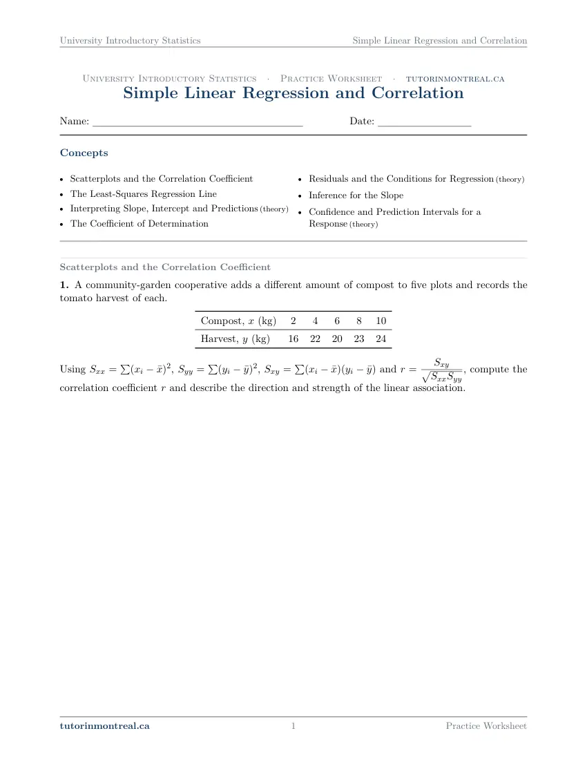
   This question is built around a diagram or a table of values. Open it in the PDF.

2. Q2Scatterplots and the Correlation Coefficient

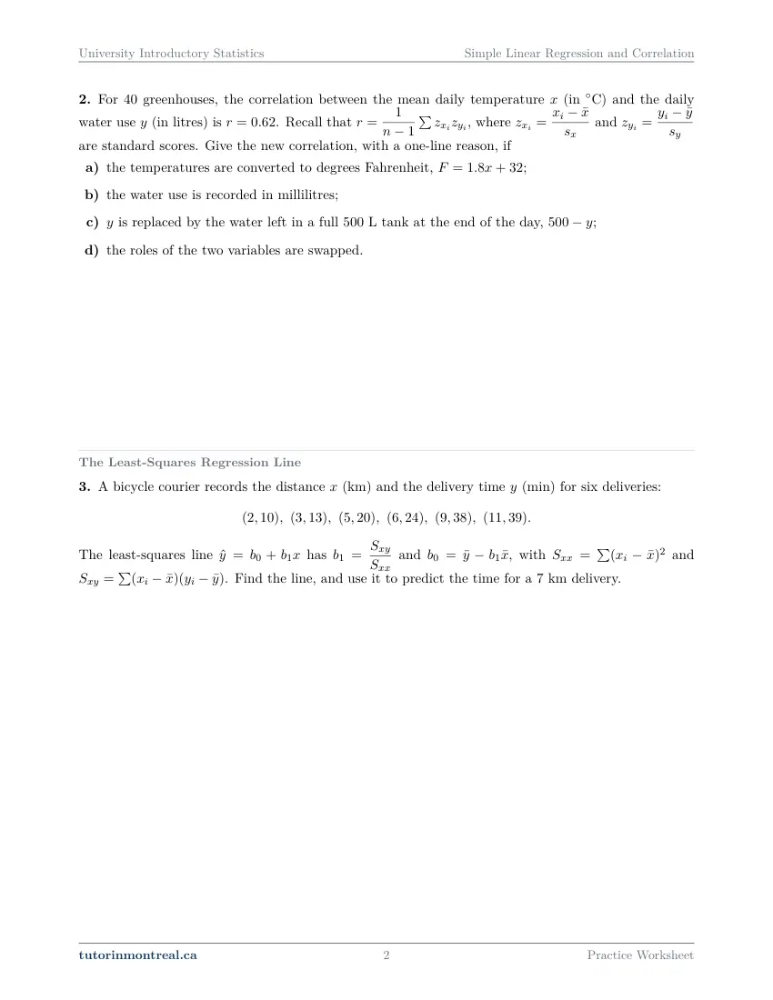
   For $40$ greenhouses, the correlation between the mean daily temperature $x$ (in ${}^{\circ }$C) and the daily water use $y$ (in litres) is $r=0.62$. Recall that $r={\displaystyle \frac{1}{n-1}}\sum z_{x_i}{z}_{y_i}$, where $z_{x_i}={\displaystyle \frac{x_i-\overline{x}}{s_x}}$ and $z_{y_i}={\displaystyle \frac{y_i-\overline{y}}{s_y}}$ are standard scores. Give the new correlation, with a one-line reason, if

   1. the temperatures are converted to degrees Fahrenheit, $F=1.8x+32$;
   2. the water use is recorded in millilitres;
   3. $y$ is replaced by the water left in a full $500$ L tank at the end of the day, $500-y$;
   4. the roles of the two variables are swapped.
3. Q3The Least-Squares Regression Line

   A bicycle courier records the distance $x$ (km) and the delivery time $y$ (min) for six deliveries: $$(2,10),(3,13),(5,20),(6,24),(9,38),(11,39).$$ The least-squares line $\widehat{y}=b_0+b_{1}x$ has $b_1={\displaystyle \frac{S_{xy}}{S_{xx}}}$ and $b_0=\overline{y}-b_1\overline{x}$, with $S_{xx}=\sum (x_i-\overline{x}{)}^2$ and $S_{xy}=\sum (x_i-\overline{x})(y_i-\overline{y})$. Find the line, and use it to predict the time for a $7$ km delivery.

4. Q4The Least-Squares Regression Line

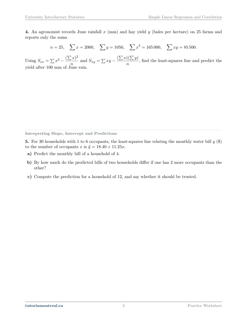
   An agronomist records June rainfall $x$ (mm) and hay yield $y$ (bales per hectare) on $25$ farms and reports only the sums $$n=25,\sum x=2000,\sum y=1050,\sum x^2=165000,\sum xy=85500.$$ Using $S_{xx}=\sum x^2-{\displaystyle \frac{(\sum x{)}^2}{n}}$ and $S_{xy}=\sum xy-{\displaystyle \frac{(\sum x)(\sum y)}{n}}$, find the least-squares line and predict the yield after $100$ mm of June rain.

5. Q5Interpreting Slope, Intercept and Predictions

   For $30$ households with $1$ to $6$ occupants, the least-squares line relating the monthly water bill $y$ ($) to the number of occupants $x$ is $\widehat{y}=18.40+11.25x$.

   1. Predict the monthly bill of a household of $4$.
   2. By how much do the predicted bills of two households differ if one has $2$ more occupants than the other?
   3. Compute the prediction for a household of $12$, and say whether it should be trusted.
6. Q6The Coefficient of Determination

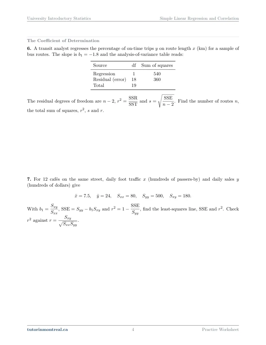
   This question is built around a diagram or a table of values. Open it in the PDF.

7. Q7The Coefficient of Determination

   For $12$ cafés on the same street, daily foot traffic $x$ (hundreds of passers-by) and daily sales $y$ (hundreds of dollars) give $$\overline{x}=7.5,\overline{y}=24,S_{xx}=80,S_{yy}=500,S_{xy}=180.$$ With $b_1={\displaystyle \frac{S_{xy}}{S_{xx}}}$, $\text{SSE}=S_{yy}-b_1{S}_{xy}$ and $r^2=1-{\displaystyle \frac{\text{SSE}}{S_{yy}}}$, find the least-squares line, SSE and $r^2$. Check $r^2$ against $r={\displaystyle \frac{S_{xy}}{\sqrt{S_{xx}{S}_{yy}}}}$.

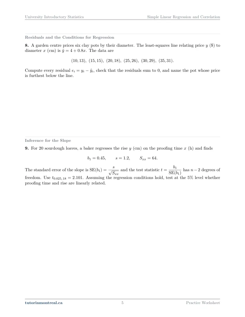
8. Q8Residuals and the Conditions for Regression

   A garden centre prices six clay pots by their diameter. The least-squares line relating price $y$ ($) to diameter $x$ (cm) is $\widehat{y}=4+0.8x$. The data are $$(10,13),(15,15),(20,18),(25,26),(30,29),(35,31).$$ Compute every residual $e_i=y_i-{\widehat{y}}_i$, check that the residuals sum to $0$, and name the pot whose price is furthest below the line.

9. Q9Inference for the Slope

   For $20$ sourdough loaves, a baker regresses the rise $y$ (cm) on the proofing time $x$ (h) and finds $$b_1=0.45,s=1.2,S_{xx}=64.$$ The standard error of the slope is $SE(b_1)={\displaystyle \frac{s}{\sqrt{S_{xx}}}}$ and the test statistic $t={\displaystyle \frac{b_1}{SE(b_1)}}$ has $n-2$ degrees of freedom. Use $t_{0.025,18}=2.101$. Assuming the regression conditions hold, test at the $5\%$ level whether proofing time and rise are linearly related.

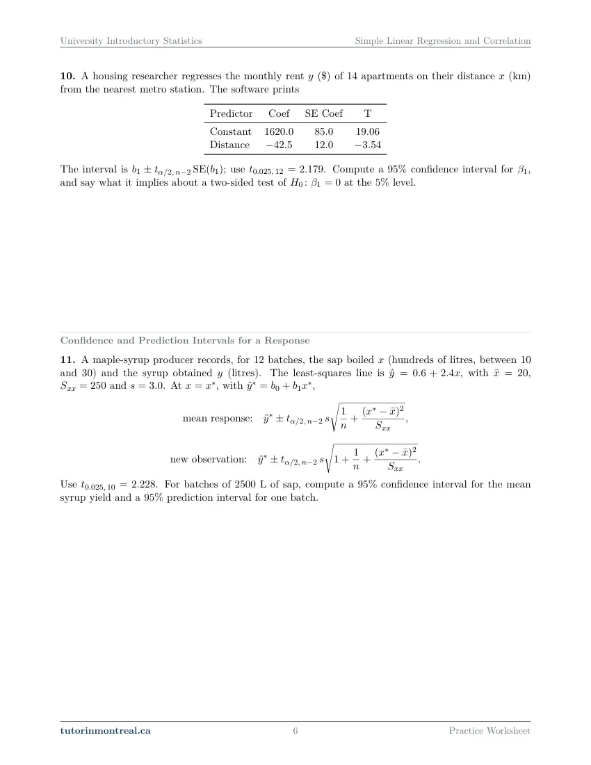
10. Q10Inference for the Slope

    This question is built around a diagram or a table of values. Open it in the PDF.

11. Q11Confidence and Prediction Intervals for a Response

    A maple-syrup producer records, for $12$ batches, the sap boiled $x$ (hundreds of litres, between $10$ and $30$) and the syrup obtained $y$ (litres). The least-squares line is $\widehat{y}=0.6+2.4x$, with $\overline{x}=20$, $S_{xx}=250$ and $s=3.0$. At $x=x^{*}$, with ${\widehat{y}}^{*}=b_0+b_1{x}^{*}$, $$\text{mean response:}{\widehat{y}}^{*}\pm t_{\alpha /2,n-2}s\sqrt{\frac{1}{n}+\frac{(x^{*}-\overline{x}{)}^2}{S_{xx}}},$$ $$\text{new observation:}{\widehat{y}}^{*}\pm t_{\alpha /2,n-2}s\sqrt{1+\frac{1}{n}+\frac{(x^{*}-\overline{x}{)}^2}{S_{xx}}}.$$ Use $t_{0.025,10}=2.228$. For batches of $2500$ L of sap, compute a $95\%$ confidence interval for the mean syrup yield and a $95\%$ prediction interval for one batch.

12. Q12Synthesis — drawing on several topics in this unit

    A bakery records the number of staff $x$ on five morning shifts and the trays of pastries $y$ finished by 9 a.m.: $$(1,9),(2,8),(3,12),(4,16),(5,15).$$ Use $b_1={\displaystyle \frac{S_{xy}}{S_{xx}}}$, $b_0=\overline{y}-b_1\overline{x}$, $s=\sqrt{{\displaystyle \frac{\text{SSE}}{n-2}}}$, $SE(b_1)={\displaystyle \frac{s}{\sqrt{S_{xx}}}}$, and $t_{0.025,3}=3.182$.

    1. Find the least-squares line.
    2. Compute the residuals, SSE and $r^2=1-{\displaystyle \frac{\text{SSE}}{S_{yy}}}$.
    3. Assuming the regression conditions hold, test $H_0:{\beta }_1=0$ against $H_a:{\beta }_1\ne 0$ at the $5\%$ level.

The 8 challenge problems for this topic are a separate, paid sheet and are not reproduced here.

How to do every concept on this sheet

This is the part worksheet sites usually leave out. Below is the actual reasoning behind each group of questions — not a full solution set, the decisions that get you to one. Read it before you start, or after you get stuck.

Scatterplots and the correlation coefficient

r measures one thing only: how closely the points cluster about a straight line, and in which direction. It is built from deviations, and every quantity on this sheet is a sum of products of deviations.

Q2 asks nothing arithmetical at all: it hands you a correlation for forty greenhouses and four changes to the data, and wants the new correlation with a one-line reason for each. Work from the standard-score form of r, which the question states.

For each part, ask what the change does to the standard scores. Adding a constant shifts the values and the mean together, so every deviation is untouched. Multiplying by a positive constant multiplies deviation and standard deviation alike, so each z is unchanged. Multiplying by a negative constant leaves the size of each z alone and reverses its sign — and the sum of products then reverses with it. And the defining formula treats the two variables symmetrically, which settles the last part without any computation. Reason from the z scores every time; guessing from the story is how this question is lost.

The least-squares regression line

The line is the one making the sum of squared vertical distances from the points as small as possible. In this course it comes from the same sums as r, and the slope is read off first.

Q3 gives six pairs of distances and delivery times: build the deviation table exactly as for Q1, take the slope from Sxy and Sxx, then the intercept from the two means. Because b₀ is found from b₁, a slope rounded early poisons the intercept — carry the slope to more decimal places than the answer needs, and round once at the end. The prediction asked for is the substitution of one value into the finished line.

Q4 gives no pairs — only n and four sums for twenty-five farms — which is how a regression is usually reported. The computational forms below are algebraically the same as the deviation forms, so nothing new is being calculated, only a different route to Sxx and Sxy.

Interpreting slope, intercept and predictions

Q5 supplies a fitted line for thirty households and asks for no fitting at all — only for what the line says. Three readings, each a sentence with units in it.

The coefficient of determination

r² is the share of the variation in y that the line accounts for. It comes either from the sums of squares or, squared back, from r itself.

Q6 gives an analysis-of-variance table for a set of bus routes and asks you to work outwards from it. The residual degrees of freedom are n − 2, so the df column fixes the sample size before anything else; the total sum of squares is the sum of the two rows above it, which is why the table leaves that cell blank. Then r² is a ratio of two entries, and s — the typical size of a residual, in the units of y — divides SSE by its own degrees of freedom, never by n.

Q7 comes at the same quantities from summary values for twelve cafés. Here SSE is got without residuals at all, from SSE = Syy − b₁Sxy, and r² from 1 − SSE/Syy. The final instruction is the point of the question: compute r from Sxy and the root of Sxx·Syy, square it, and see that the two routes meet. An agreement to several decimal places is a check; a disagreement means one of the S values was used in the wrong slot.

Residuals and the conditions for regression

A residual is what the line did not explain about one observation: the vertical gap between the point and the line, signed.

Q8 gives six clay pots and the fitted line, and asks for every residual. Work down the list: predict, subtract, keep the sign. The sum being zero is a property of the least-squares fit, so when your column does not add to zero the error is in the arithmetic, not in the data — that is why the question asks for the check before anything else.

Behind every inference later on this sheet sit four conditions, and a residual plot — residuals against x — is how each is examined: the relationship is linear (no curved band of points), the spread of the residuals is the same all along (no funnel), the observations are independent, and the residuals are roughly normal about zero. A pattern in that plot names the condition that is in trouble, which is why the inference questions state that the conditions hold before asking for a test.

Inference for the slope

The fitted slope is an estimate of an unknown slope β₁, and a different sample would give a different b₁. Its standard error measures that variability, and everything inferential for a regression is built on it.

Q10 works from a printed table of coefficients for fourteen apartments, and the reading is the first decision: the row for the explanatory variable, not the row for the constant, carries the slope and its standard error. Build the interval from the general form, with the t value the question supplies.

Confidence and prediction intervals for a response

Two different questions live at the same x*, and they have different answers. One asks for the average response of all units at that value; the other asks for one new unit. The second must allow for that unit's own scatter about the line, which is the extra 1 under the root.

Q11 gives twelve batches of sap, the fitted line, x̄, Sxx and s. Two things decide the question before any arithmetic. First, the units: x is counted in hundreds of litres and the batch size is quoted in litres, so convert before substituting, or every number afterwards is wrong. Second, which interval each part is asking for — the wording "the mean syrup yield" against "one batch" is the whole distinction. Compute ŷ* once; only the root differs between the two.

The synthesis question

Q12 runs the whole sheet on five morning shifts at a bakery, and its three parts are the three chapters in order: fit the line with the slope-and-intercept formulas, then the residuals, SSE and r², then the t test for the slope against a two-sided alternative at the stated level.

Two things make it harder than its parts. The sample is small, so the degrees of freedom are few and the supplied critical value is correspondingly large — read it as a reminder of how little a handful of points can settle. And part (b) feeds part (c): SSE gives s, s gives SE(b₁), and SE(b₁) gives t, so a residual mis-subtracted in the middle carries all the way to the conclusion. Recompute r² the other way, from r, before moving on, and finish with a sentence about staff and trays rather than about t.

Preview all 7 pages

Click any page to open the full PDF.

Getting the most out of it

Set the table up before touching a formula

Means at the top, then columns for the two deviations, their squares and their product. Every quantity on this topic — r, b₁, SSE, r² — is a combination of those three totals, so one careful table answers a whole question and gives you the add-to-zero check for free.

Say the slope out loud, with units

"One more occupant is associated with so many more dollars on the predicted bill" is the form the interpretation questions want. Numbers without units and without the words "is associated with" are what lose the interpretation marks that every part of this chapter carries.

Check the x you are predicting at

Before reporting any prediction or interval, compare the value of x with the range the data covered. Inside it, the line is evidence; outside it, the arithmetic still works and the prediction does not. Q5 and Q11 both turn on this, and an exam question rarely warns you.

Reach for the second route as a check

r² from the sums of squares against r² from r; the point of means substituted into the line; the residual column adding to zero; the interval compared with the test. This topic is unusually rich in checks that cost one line, and using them is faster than finding the slip later.

End on the situation, not the statistic

Every question here asks for tomatoes, deliveries, bus routes, loaves or rent, and the marks at the end belong to the sentence that answers in those terms at the stated level. Write the number, then write what it means about the two variables.

Common questions