University Introductory Statistics — Discrete Random Variables Worksheet

7 of the 11 questions

Each question targets one named concept from the sheet. Read them here, or print the PDF — it has working space under each one. 7 of the 11 questions are printed below. The other 4 are built on a diagram or a table of values that does not translate to the page, so they are in the free PDF — marked below where they would have come.

1. Q1Probability Mass Functions and Cumulative Distributions

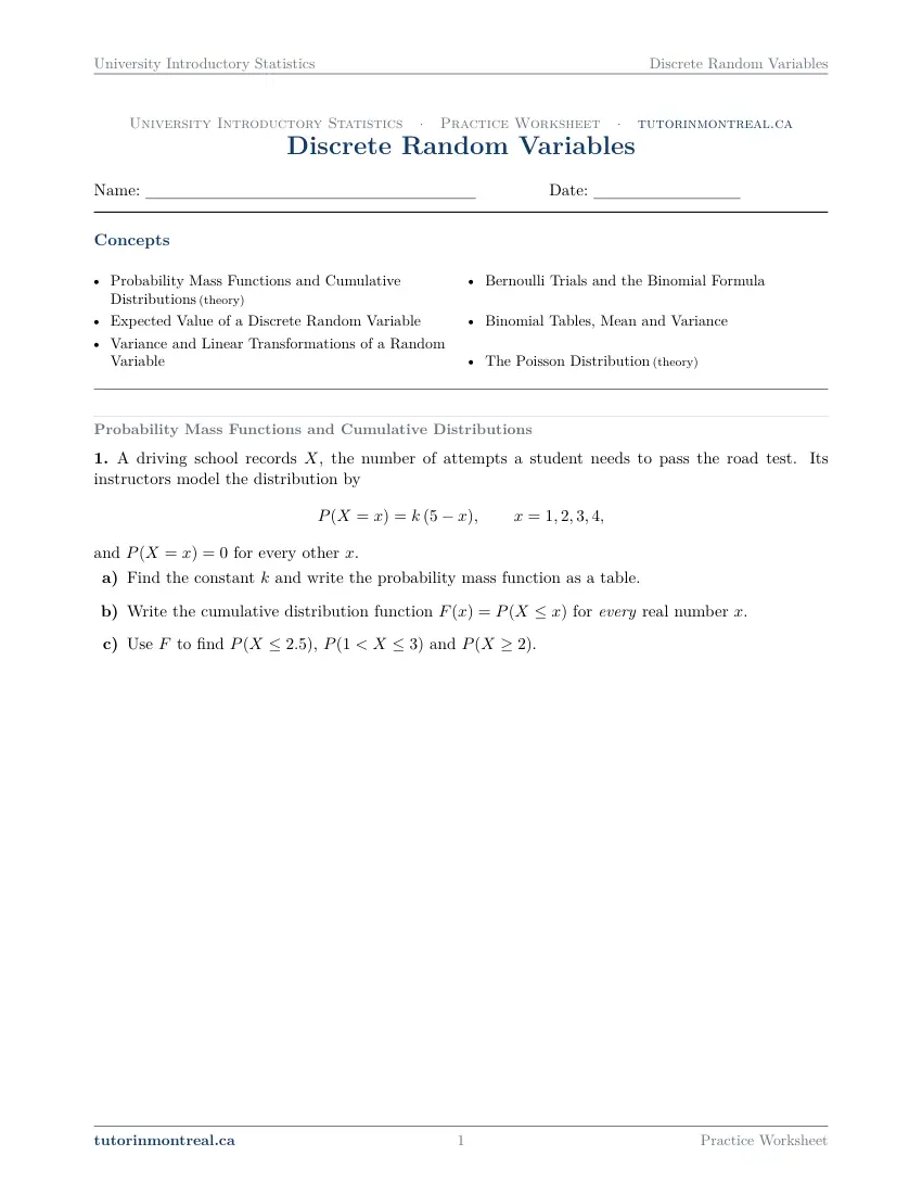
   A driving school records $X$, the number of attempts a student needs to pass the road test. Its instructors model the distribution by $$P(X=x)=k(5-x),x=1,2,3,4,$$ and $P(X=x)=0$ for every other $x$.

   1. Find the constant $k$ and write the probability mass function as a table.
   2. Write the cumulative distribution function $F(x)=P(X\le x)$ for every real number $x$.
   3. Use $F$ to find $P(X\le 2.5)$, $P(1<X\le 3)$ and $P(X\ge 2)$.
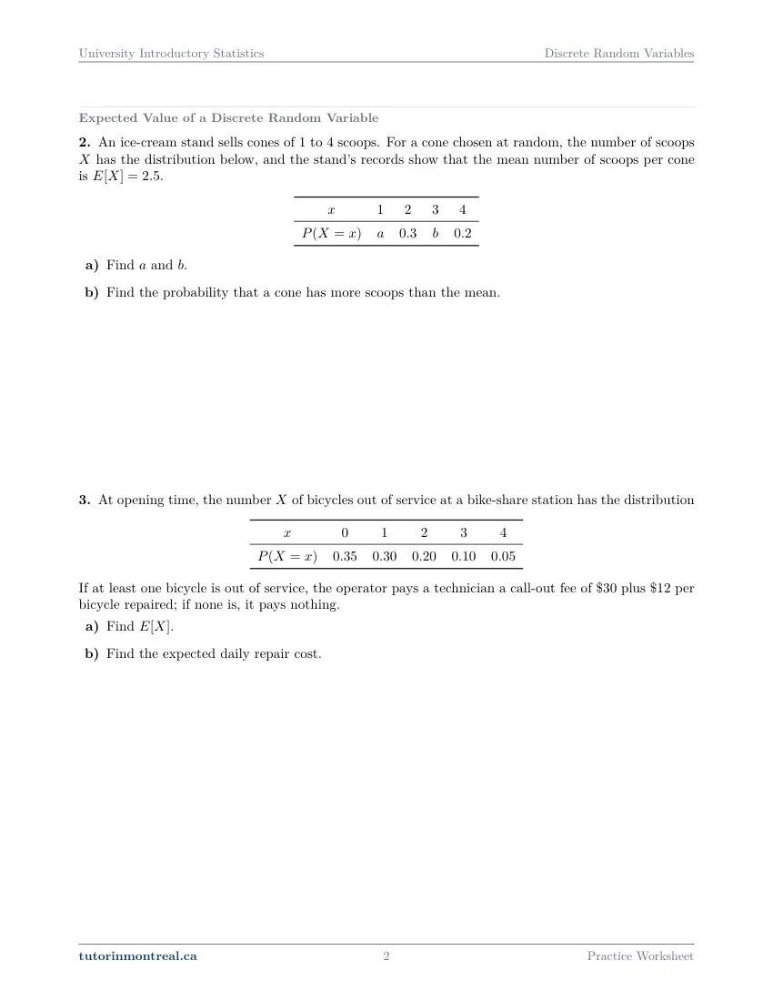
2. Q2Expected Value of a Discrete Random Variable

   This question is built around a diagram or a table of values. Open it in the PDF.

3. Q3Expected Value of a Discrete Random Variable

   This question is built around a diagram or a table of values. Open it in the PDF.

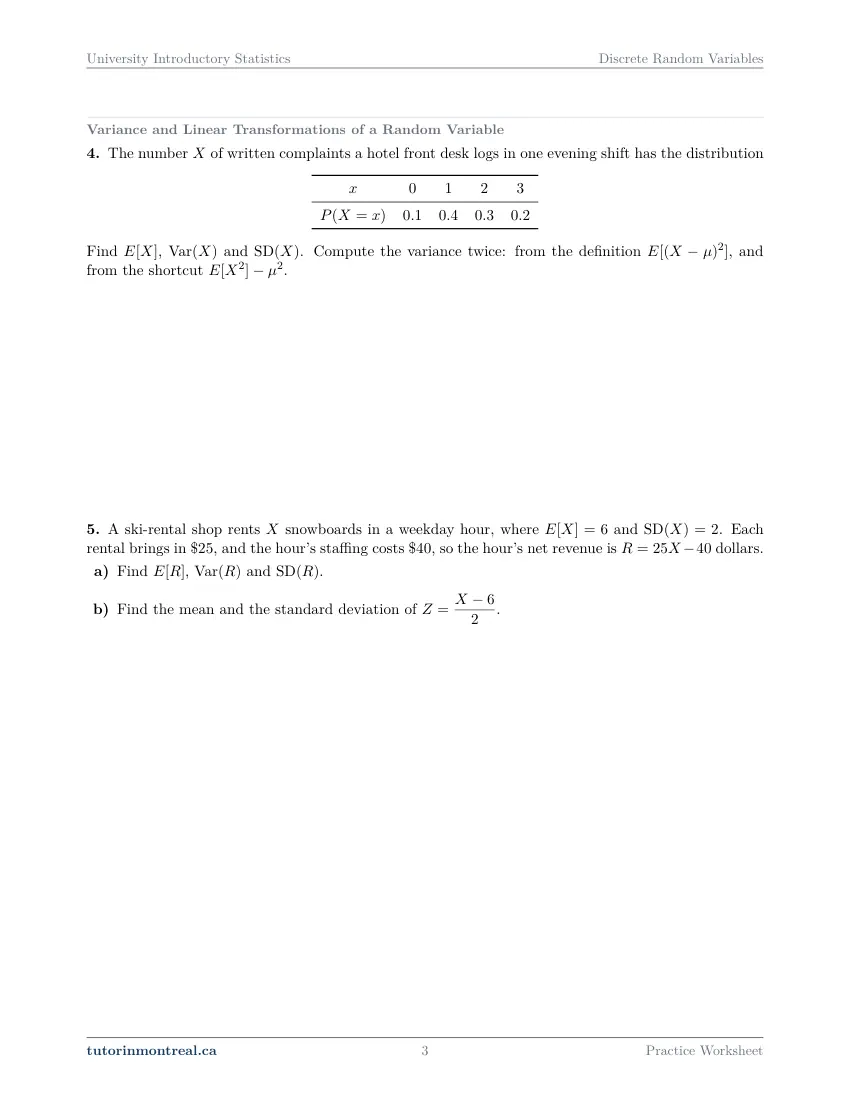
4. Q4Variance and Linear Transformations of a Random Variable

   This question is built around a diagram or a table of values. Open it in the PDF.

5. Q5Variance and Linear Transformations of a Random Variable

   A ski-rental shop rents $X$ snowboards in a weekday hour, where $E[X]=6$ and $SD(X)=2$. Each rental brings in $25, and the hour's staffing costs $40, so the hour's net revenue is $R=25X-40$ dollars.

   1. Find $E[R]$, $Var(R)$ and $SD(R)$.
   2. Find the mean and the standard deviation of $Z={\displaystyle \frac{X-6}{2}}$.
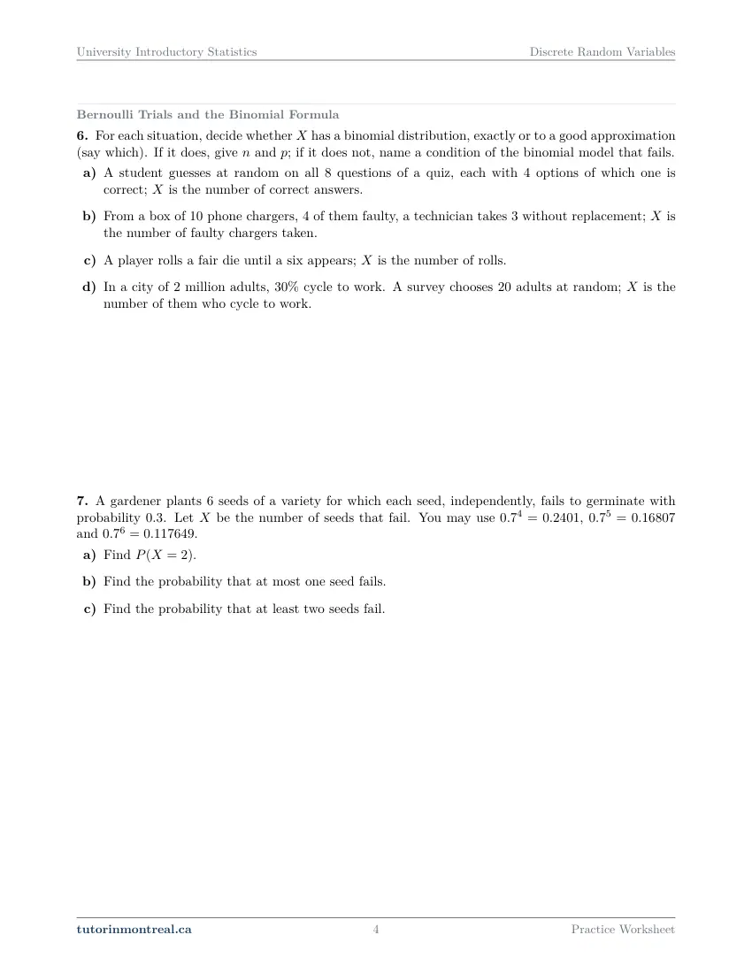
6. Q6Bernoulli Trials and the Binomial Formula

   For each situation, decide whether $X$ has a binomial distribution, exactly or to a good approximation (say which). If it does, give $n$ and $p$; if it does not, name a condition of the binomial model that fails.

   1. A student guesses at random on all $8$ questions of a quiz, each with $4$ options of which one is correct; $X$ is the number of correct answers.
   2. From a box of $10$ phone chargers, $4$ of them faulty, a technician takes $3$ without replacement; $X$ is the number of faulty chargers taken.
   3. A player rolls a fair die until a six appears; $X$ is the number of rolls.
   4. In a city of $2$ million adults, $30\%$ cycle to work. A survey chooses $20$ adults at random; $X$ is the number of them who cycle to work.
7. Q7Bernoulli Trials and the Binomial Formula

   A gardener plants $6$ seeds of a variety for which each seed, independently, fails to germinate with probability $0.3$. Let $X$ be the number of seeds that fail. You may use ${0.7}^4=0.2401$, ${0.7}^5=0.16807$ and ${0.7}^6=0.117649$.

   1. Find $P(X=2)$.
   2. Find the probability that at most one seed fails.
   3. Find the probability that at least two seeds fail.
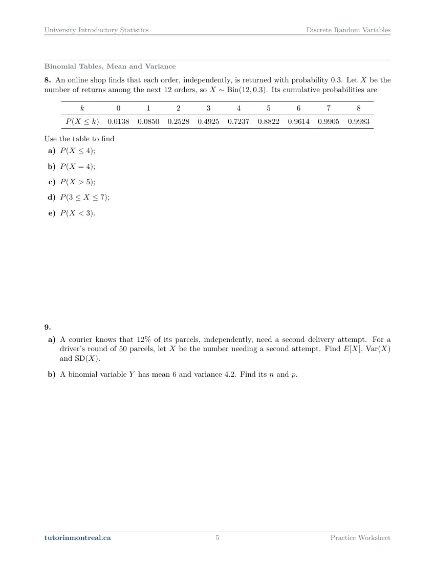
8. Q8Binomial Tables, Mean and Variance

   This question is built around a diagram or a table of values. Open it in the PDF.

9. Q9Binomial Tables, Mean and Variance
   1. A courier knows that $12\%$ of its parcels, independently, need a second delivery attempt. For a driver's round of $50$ parcels, let $X$ be the number needing a second attempt. Find $E[X]$, $Var(X)$ and $SD(X)$.
   2. A binomial variable $Y$ has mean $6$ and variance $4.2$. Find its $n$ and $p$.
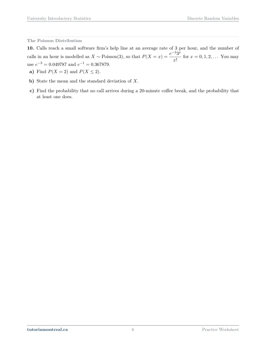
10. Q10The Poisson Distribution

    Calls reach a small software firm's help line at an average rate of $3$ per hour, and the number of calls in an hour is modelled as $X~\text{Poisson}(3)$, so that $P(X=x)={\displaystyle \frac{e^{-3}{3}^x}{x!}}$ for $x=0,1,2,\dots$ You may use $e^{-3}=0.049787$ and $e^{-1}=0.367879$.

    1. Find $P(X=2)$ and $P(X\le 2)$.
    2. State the mean and the standard deviation of $X$.
    3. Find the probability that no call arrives during a $20$-minute coffee break, and the probability that at least one does.
11. Q11Synthesis — drawing on several topics in this unit

    An airport shuttle van has $10$ passenger seats. Because some passengers do not turn up, the company accepts $11$ bookings for each trip. Each booked passenger turns up with probability $0.9$, independently of the others. Let $X$ be the number who turn up. You may use $P(X=10)=0.3835$ and $P(X=11)=0.3138$.

    1. Name the distribution of $X$, with its parameters, and find $E[X]$ and $SD(X)$.
    2. Find the probability that the van is overbooked (a passenger who turns up has no seat).
    3. Find the probability that the van leaves with at least one empty seat.
    4. Let $B$ be the number of passengers left without a seat. Write the distribution of $B$ and find $E[B]$.

The 7 challenge problems for this topic are a separate, paid sheet and are not reproduced here.

How to do every concept on this sheet

This is the part worksheet sites usually leave out. Below is the actual reasoning behind each group of questions — not a full solution set, the decisions that get you to one. Read it before you start, or after you get stuck.

Probability mass functions and cumulative distributions

A discrete random variable is a rule that attaches a number to each outcome. Its probability mass function lists the values it can take and the probability of each, and it is a legitimate model only when every probability is between 0 and 1 and the whole list adds to 1. That second condition is not decoration — it is the equation that pins down an unknown constant.

Q1 gives a formula with an unknown multiplier in it and a short list of allowed values. Write the four probabilities in terms of the constant, add them, set the sum equal to 1, and solve the one-line equation; only then is the table worth writing out. Finishing with a table rather than the formula is part of the question, and it is also the fastest way to check your own constant — four numbers that do not add to 1 are visible at a glance.

Q1(c) then asks for three probabilities read off F rather than off the table, which is the skill the sheet is really after. Translate each one into F before touching a number:

The strictness of an inequality matters here in a way it never does for a continuous model. P(X < a) and P(X ≤ a) differ by the whole jump at a, so a question written with < is not the same question as one written with ≤. When the point asked about is not one of the values of X, it sits on a flat stretch and F takes the value it already had.

Expected value of a discrete random variable

The expected value is the average of the values, weighted by their probabilities — the balance point of the mass function, not necessarily a value the variable can ever take.

Q2 runs that definition backwards. Two probabilities in the table are unknown and two facts are given: the probabilities add to 1, and the mean is stated. Write each fact as an equation in the two unknowns and solve the pair; a negative probability or one above 1 at the end means an arithmetic slip, not an unusual answer. Q2(b) then asks for a probability described in words — more scoops than the mean. Decide first which values of X satisfy the description, strictly, and add only their probabilities.

In practice that means one extra column beside the table: for each value of X work out what the cost would be, then weight those costs by the same probabilities. Q3(a) is the plain mean of X and is worth doing first, because it is one of the columns you need anyway.

Variance, standard deviation and the shortcut

Variance is the expected squared distance from the mean, and the standard deviation is its square root, back in the units of X.

Q4 asks for both routes on the same table, on purpose. The definition needs a column of (x − μ)² and is the version that makes the meaning visible; the shortcut needs a column of x² and is the version you will use under time pressure. They are algebraically the same quantity, so two different answers mean an error in one column, and finding which one is the point of doing it twice.

Linear transformations of a random variable

Shifting a variable moves its centre and leaves its spread alone; scaling it moves both, and the variance moves by the square of the scale factor.

Q5 supplies a mean and a standard deviation and never a table, which is the signal that these three rules are the whole method — there is nothing to sum. In Q5(a) the net revenue is a fixed amount per rental minus a fixed hourly staffing cost, so read a and b off the expression and apply each rule in turn. The constant b is the trap: it moves the mean and does nothing at all to the variance or the standard deviation.

Bernoulli trials and the binomial formula

The binomial model counts successes in a fixed number of independent trials that all have the same success probability. All four of those conditions have to hold before the formula means anything.

Q6 is four situations and no arithmetic whatsoever. For each one the answer has a fixed shape: either the four conditions hold — exactly, or well enough to be a good approximation, and the question asks you to say which — and then you state n and p; or one condition fails, and you name it. Work through the list above in order rather than deciding by feel, and say where each number comes from: n is what the situation repeats, p is the probability of the thing being counted on a single trial.

Q7 gives you three powers to save arithmetic, which is a hint about the shape of the work: the parts that are quick are the ones built from a small number of terms. Q7(b) is a sum of two terms straight from the formula. Q7(c) describes an event whose complement is exactly the event in Q7(b), and subtracting from 1 is much shorter than adding five terms — the general move whenever a question says "at least".

Binomial tables, mean and variance

A printed cumulative table gives P(X ≤ k) and nothing else, so every question has to be rewritten in that form before you look anything up. Q8 is five rewritings and five lookups.

The mean and variance of a binomial variable need no table and no sum, because the model already fixes them:

Q9(a) applies those three to a stated n and p. Q9(b) runs them backwards: two equations, two unknowns, and the quickest route is to divide the variance by the mean, because everything but one factor cancels and p follows from what is left. Then recover n from the mean. Finish by checking that p lies between 0 and 1 and that n is a whole number — if either fails, no binomial variable has those two moments.

The Poisson distribution

The Poisson model counts events in a fixed interval of time or space when they occur at a constant average rate, independently of one another, and there is no natural n to count out of. One parameter does all the work.

Q10 states the rate per hour and supplies the exponential values you need, so the arithmetic is short and the decisions are everything. Q10(a) is one term of the formula and then a sum of the terms up to a stated value. Q10(b) is a statement, not a computation: the mean and the variance of a Poisson variable are the same number, which is why the standard deviation is a square root of it — say so rather than adding a column.

The synthesis question

Q11 is the overbooking problem, and it uses most of the sheet at once. Q11(a) asks you to name the distribution with its parameters before anything else: run the four conditions over the wording, read n and p off it, and then the mean and standard deviation are the binomial formulas rather than a table of eleven rows. The two probabilities printed in the question are there because the parts that follow need exactly those and no others — a sign that each part should reduce to a short combination of them.

Q11(b) and (c) are both translations before they are computations. Say in plain words which values of X describe an overbooked van, and which describe a van leaving with a seat free; the two descriptions between them should account for every possible value, which is the check. Then rewrite each as a cumulative or complementary probability, exactly as in Q8.

Preview all 7 pages

Click any page to open the full PDF.

Getting the most out of it

Draw the table, even when you are given a formula

Values across the top, probabilities beneath, then one extra row for whatever the question needs — x·P(x), x², (x − μ)², a cost. Almost every question in this set is one more row on a table you have already written, and a table that does not add to 1 stops you before the error spreads into the mean.

Translate the words before you compute

"At least", "more than", "fewer than", "at most", "more than the mean": write each as an inequality on X, then as an expression in F or in the mass function, and only then reach for the calculator. On a whole-number variable, moving between < and ≤ changes the answer, and it is where this chapter's marks are lost.

Name the model before using its formulas

np, np(1 − p) and the single Poisson parameter are shortcuts that are only valid once the model is justified. Write the conditions you checked, in one line, above the formula. An exam question that says "find the probability" is also silently asking you to defend the model you chose.

Reach for the complement

"At least one", "more than five", "not all": write the complement beside the event and count the terms each version needs. The complement usually wins, and with a cumulative table it is one subtraction rather than a column of additions.

Sanity-check every answer against the table

A probability outside 0 to 1, a mean outside the range of values, a standard deviation larger than that range, a variance carrying the units of X: each is a thirty-second check and each catches a different mistake. Do them before writing the sentence that interprets the result.

Common questions