University Introductory Statistics — Continuous Distributions and the Normal Model Worksheet

8 of the 10 questions

Each question targets one named concept from the sheet. Read them here, or print the PDF — it has working space under each one. 8 of the 10 questions are printed below. The other 2 are built on a diagram or a table of values that does not translate to the page, so they are in the free PDF — marked below where they would have come.

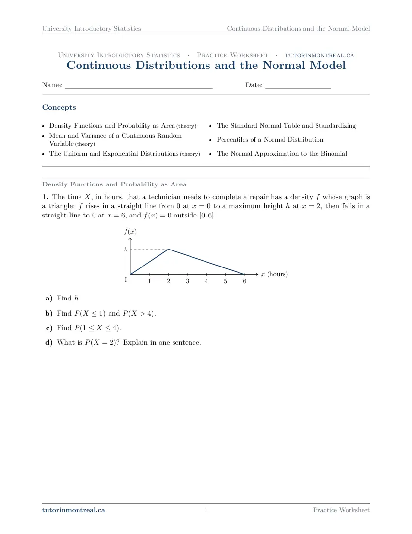
1. Q1Density Functions and Probability as Area

   This question is built around a diagram or a table of values. Open it in the PDF.

2. Q2Mean and Variance of a Continuous Random Variable

   The time $X$, in minutes, that a barista takes to prepare an order has a triangular density: it rises in a straight line from $0$ at $x=2$ to a peak at $x=5$, then falls in a straight line to $0$ at $x=8$, and is $0$ outside $[2,8]$.

   1. Find the height of the peak.
   2. Find $E[X]$, and justify your answer without any formula.
   3. For a triangular density on $[a,b]$ with its peak at $c$, $$Var(X)=\frac{a^2+b^2+c^2-ab-ac-bc}{18}.$$ Find $Var(X)$ and $SD(X)$.
   4. Find $P(X>7)$.
3. Q3The Uniform and Exponential Distributions
   1. A ferry leaves every $20$ minutes, and a passenger who ignores the timetable arrives at a random moment, so the wait $W$, in minutes, is uniform on $[0,20]$. Find $P(W>15)$ and $P(5<W<12)$.
   2. For a uniform variable on $[a,b]$, $E[W]={\displaystyle \frac{a+b}{2}}$ and $Var(W)={\displaystyle \frac{(b-a{)}^2}{12}}$. Find the mean and standard deviation of the wait.
   3. At a bike-share dock, the time $T$, in minutes, between two returns is exponential with mean $4$ minutes, so $P(T\le t)=1-e^{-t/4}$ for $t\ge 0$. Find $P(T>8)$ and $P(2<T\le 6)$, exactly and to four decimals. Use $e^{-0.5}=0.6065$, $e^{-1.5}=0.2231$, $e^{-2}=0.1353$.
4. Q4The Standard Normal Table and Standardizing

   Let $Z$ be a standard normal variable. The table available gives $P(Z<z)$ for $z\ge 0$ only: $$P(Z<0.62)=0.7324,P(Z<0.84)=0.7995,P(Z<1.37)=0.9147,P(Z<1.50)=0.9332.$$ Find:

   1. $P(Z<1.37)$;
   2. $P(Z>-0.84)$;
   3. $P(-1.50<Z<0.62)$;
   4. $P(|Z|>1.37)$.
5. Q5The Standard Normal Table and Standardizing

   This question is built around a diagram or a table of values. Open it in the PDF.

6. Q6Percentiles of a Normal Distribution

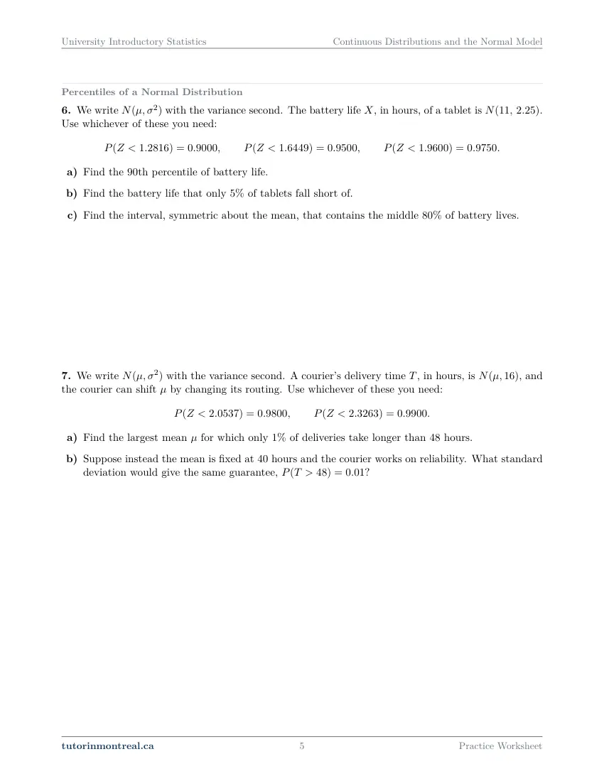
   We write $N(\mu ,{\sigma }^2)$ with the variance second. The battery life $X$, in hours, of a tablet is $N(11,2.25)$. Use whichever of these you need: $$P(Z<1.2816)=0.9000,P(Z<1.6449)=0.9500,P(Z<1.9600)=0.9750.$$

   1. Find the $90$th percentile of battery life.
   2. Find the battery life that only $5\%$ of tablets fall short of.
   3. Find the interval, symmetric about the mean, that contains the middle $80\%$ of battery lives.
7. Q7Percentiles of a Normal Distribution

   We write $N(\mu ,{\sigma }^2)$ with the variance second. A courier's delivery time $T$, in hours, is $N(\mu ,16)$, and the courier can shift $\mu$ by changing its routing. Use whichever of these you need: $$P(Z<2.0537)=0.9800,P(Z<2.3263)=0.9900.$$

   1. Find the largest mean $\mu$ for which only $1\%$ of deliveries take longer than $48$ hours.
   2. Suppose instead the mean is fixed at $40$ hours and the courier works on reliability. What standard deviation would give the same guarantee, $P(T>48)=0.01$?
8. Q8The Normal Approximation to the Binomial

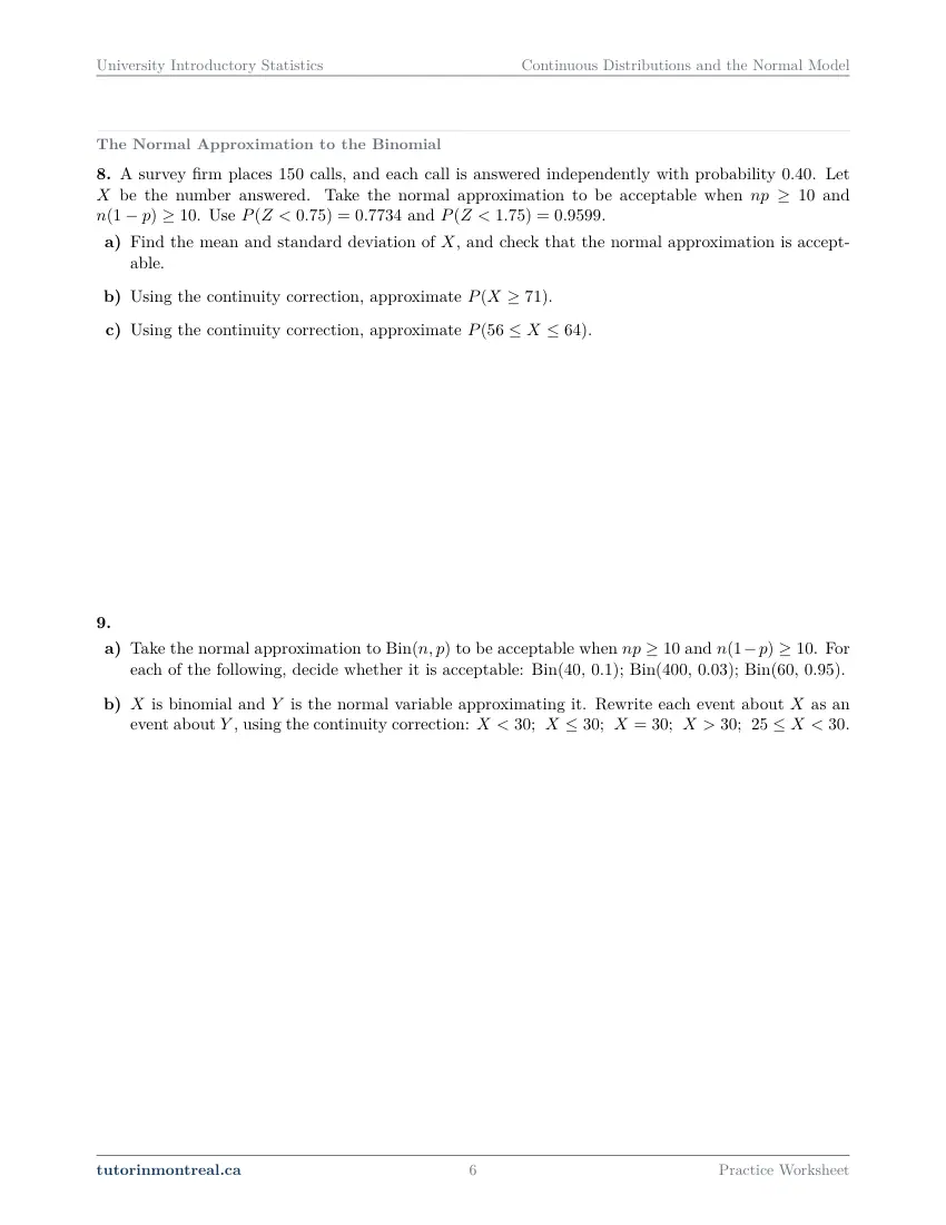
   A survey firm places $150$ calls, and each call is answered independently with probability $0.40$. Let $X$ be the number answered. Take the normal approximation to be acceptable when $np\ge 10$ and $n(1-p)\ge 10$. Use $P(Z<0.75)=0.7734$ and $P(Z<1.75)=0.9599$.

   1. Find the mean and standard deviation of $X$, and check that the normal approximation is acceptable.
   2. Using the continuity correction, approximate $P(X\ge 71)$.
   3. Using the continuity correction, approximate $P(56\le X\le 64)$.
9. Q9The Normal Approximation to the Binomial
   1. Take the normal approximation to $\text{Bin}(n,p)$ to be acceptable when $np\ge 10$ and $n(1-p)\ge 10$. For each of the following, decide whether it is acceptable: $\text{Bin}(40,0.1)$; $\text{Bin}(400,0.03)$; $\text{Bin}(60,0.95)$.
   2. $X$ is binomial and $Y$ is the normal variable approximating it. Rewrite each event about $X$ as an event about $Y$, using the continuity correction: $X<30$;\; $X\le 30$;\; $X=30$;\; $X>30$;\; $25\le X<30$.
10. Q10Synthesis — drawing on several topics in this unit

    We write $N(\mu ,{\sigma }^2)$ with the variance second. The volume of paint in a tin labelled $1$ litre is $N(1000,64)$ millilitres, and a tin is underfilled if it holds less than $988$~mL. Tins are filled independently. Take the normal approximation to the binomial to be acceptable when $np\ge 10$ and $n(1-p)\ge 10$. Use whichever of these you need: $P(Z<1.09)=0.8621$, $P(Z<1.18)=0.8810$, $P(Z<1.50)=0.9332$.

    1. Find the probability $p$ that a tin is underfilled.
    2. A shipment holds $500$ tins. Using the continuity correction, approximate the probability that $40$ or more of them are underfilled.

The 7 challenge problems for this topic are a separate, paid sheet and are not reproduced here.

How to do every concept on this sheet

This is the part worksheet sites usually leave out. Below is the actual reasoning behind each group of questions — not a full solution set, the decisions that get you to one. Read it before you start, or after you get stuck.

Density functions and probability as area

A discrete variable carries a probability at each value; a continuous one carries probability over intervals, as area under a curve. Two properties do all the work: the density is never negative, and the total area under it is 1. Q1 gives a triangular density as a graph with its peak height h unnamed, so the first part is the total-area property turned into an equation for h.

That is Q1(b) and Q1(c). The cut in Q1(b) falls on the rising edge in one part and on the falling edge in the other, so the two are not mirror images and each needs its own height. Q1(c) can be done directly or as 1 minus the two outer pieces you already have — do it both ways once, and the agreement is the check.

The mean and the spread of a continuous variable

Q2 is the same kind of density with a different demand: locate its centre and measure its spread. Part (a) is the total-area property again. Part (b) forbids any formula, so the justification has to come from the picture.

Q2(c) hands you the variance formula for a triangular density, so use it exactly as printed — substitute the two endpoints and the peak, and do not try to rebuild it. The standard deviation is the square root of what comes out, in the same units as X, which is why it is the number worth interpreting. Q2(d) returns to area, on the falling edge only.

The uniform and exponential distributions

Two named non-normal models, both handled without calculus. The uniform density on an interval is a flat line, so every probability is the area of a rectangle: the width of the event divided by the width of the whole interval.

Q3(a) is that ratio twice, and the second event is an interval strictly inside the range rather than a tail. Q3(b) supplies the mean and the variance of a uniform variable, so the only decisions left are substituting the endpoints the question names and remembering that the standard deviation asked for is the square root of the variance, not the variance itself.

The standard normal table and standardizing

Z is the normal variable with mean 0 and standard deviation 1, and the table in Q4 gives P(Z < z) for z ≥ 0 only. That restriction is the point of the question: every other kind of event has to be rewritten as one or more of those left-tail readings.

Q5 moves to a variable that is not standard, and its first trap is notation: N(μ, σ²) puts the variance second, so take a square root before doing anything else. The question says so explicitly, and the same warning is repeated in Q6, Q7 and Q10 because it costs more marks than any other single slip in this chapter.

Q5(a) is one standardization; Q5(b) is two, with a subtraction between them, and it also asks you to shade the region on the printed curve — do that before computing, since a shaded picture that disagrees with your arithmetic catches a reversed subtraction immediately. Q5(c) uses the 68–95–99.7 rule instead of the table: count how many standard deviations each endpoint sits from the mean, and if the count is a whole number the rule applies directly. The tick marks on the printed curve are placed at exactly those distances, so the counting is done by looking.

Percentiles: running the table backwards

Everything so far went from a value to a probability. Q6 and Q7 go the other way: the probability is given and something else is unknown. The move is always the same — write the standardized statement, match the given area to a z from the printed list, then solve.

Q6(a) asks for the value with a stated area below it. Q6(b) is worded as a shortfall rather than as a percentile, so the first job is translating "only 5% fall short of it" into an area on the correct side, which puts z below zero and calls for the symmetry step of Q4. Q6(c) is an interval symmetric about the mean holding a stated middle share: split what is left over into two equal tails, find the z that cuts off one of them, and build both endpoints with ± in one line.

Q7 keeps the probability fixed and makes a parameter the unknown. In part (a) the mean is unknown and the standard deviation is given; in part (b) the mean is fixed and the standard deviation is unknown, with the same guarantee to be met. Both parts start identically: convert the stated tail probability into the z that cuts it off, write z = (x − μ)/σ with the one unknown left in place, and solve the resulting linear equation. Part (b) is worth a sentence afterwards — the two parts are two different ways of buying the same guarantee, and saying which lever each one pulls is the interpretation the question is after.

The normal approximation to the binomial

A binomial count with a large n is tedious to compute exactly, and its histogram looks like a bell. The approximation replaces X by a normal variable with the binomial's own mean and standard deviation — but only when the distribution is not badly lopsided, which is what the size condition tests.

Q8(a) asks for both numbers and for the condition to be checked in writing, with both quantities evaluated — an approximation used without its check is incomplete even when it is justified. Q8(b) and Q8(c) then apply it to a one-sided and a two-sided event.

Q9 strips both ideas down to their mechanics. Q9(a) is three size checks and nothing else: write out both products for each one and compare each against the threshold. The three pairs (n, p) are chosen to be unalike — one has a small n, one a p near 0, one a p near 1 — and which of the two products is the binding one changes with them, so never check only np. Q9(b) is five events about X to be rewritten as events about the approximating normal variable. Take them one at a time and say each in words first ("fewer than 30", "30 or fewer"); the one stated as an equality needs the same reasoning as the inequalities, not a shortcut.

The synthesis question

Q10 chains the chapter together. Part (a) is a normal probability of the Q5 kind, with the variance given second once more. Part (b) then treats that probability as the p of a binomial count over a shipment, checks the size condition on it, and approximates a one-sided event with the continuity correction — so an error in part (a) propagates, and it is worth confirming that the probability from part (a) is plausible from the picture before building on it. The chain is the lesson: a proportion produced by a continuous model becomes the parameter of a discrete count, which is then approximated by a continuous model again.

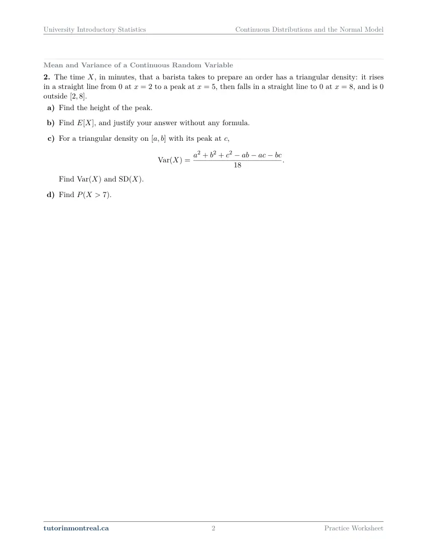
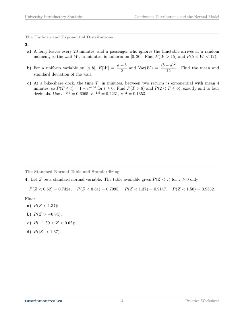
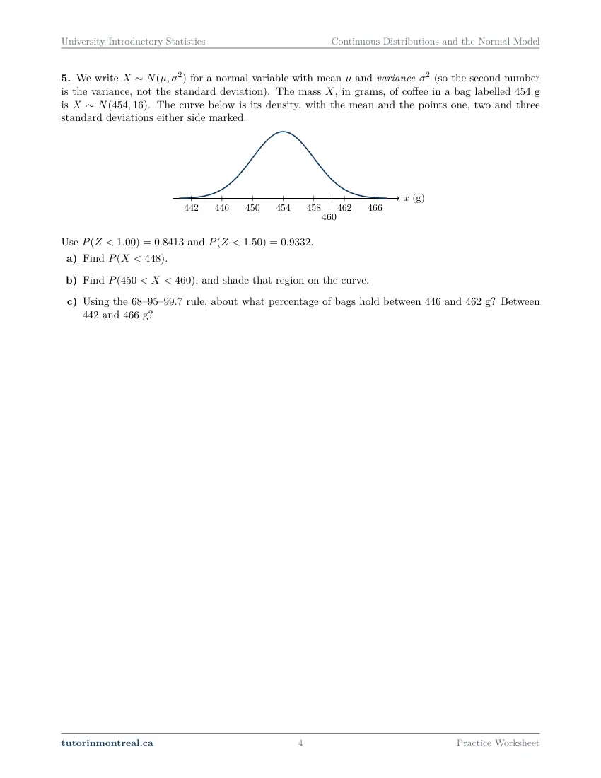
Preview all 7 pages

Click any page to open the full PDF.

Getting the most out of it

Sketch the curve before every calculation

A bell with the mean marked and the event shaded, or a triangle with the region cut into shapes: the picture decides whether you subtract, add or double, and it catches a tail taken on the wrong side faster than any re-reading of the arithmetic.

Say out loud which number the second slot holds

N(μ, σ²) is written with the variance second throughout this set. Before standardizing, write σ on its own line as the square root of that number. More marks are lost to this one habit than to the table itself.

Ask which direction the question runs

Value to probability, or probability to value? The first standardizes and looks up; the second matches an area to a z and solves for what is missing. Naming the direction first tells you which of the two templates to write down.

Check whether the variable is a count

If it counts whole things, it is discrete: the size condition has to be checked before a normal curve may be used, and the boundaries need the half-unit shift. If it measures something on a continuous scale, neither applies.

Finish with a sentence

Every number here describes something — a wait, a mass, a battery life, a count of calls. Write what it means in the context, in words, next to the number. Several parts of this set award marks for that sentence alone.

Common questions