University Introductory Statistics — Confidence Intervals Worksheet

All 10 questions

Each question targets one named concept from the sheet. Read them here, or print the PDF — it has working space under each one.

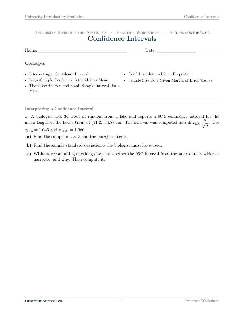
1. Q1Interpreting a Confidence Interval

   A biologist nets $36$ trout at random from a lake and reports a $90\%$ confidence interval for the mean length of the lake's trout of $(31.2,34.8)$ cm. The interval was computed as $\overline{x}\pm z_{0.05}{\displaystyle \frac{s}{\sqrt{n}}}$. Use $z_{0.05}=1.645$ and $z_{0.025}=1.960$.

   1. Find the sample mean $\overline{x}$ and the margin of error.
   2. Find the sample standard deviation $s$ the biologist must have used.
   3. Without recomputing anything else, say whether the $95\%$ interval from the same data is wider or narrower, and why. Then compute it.
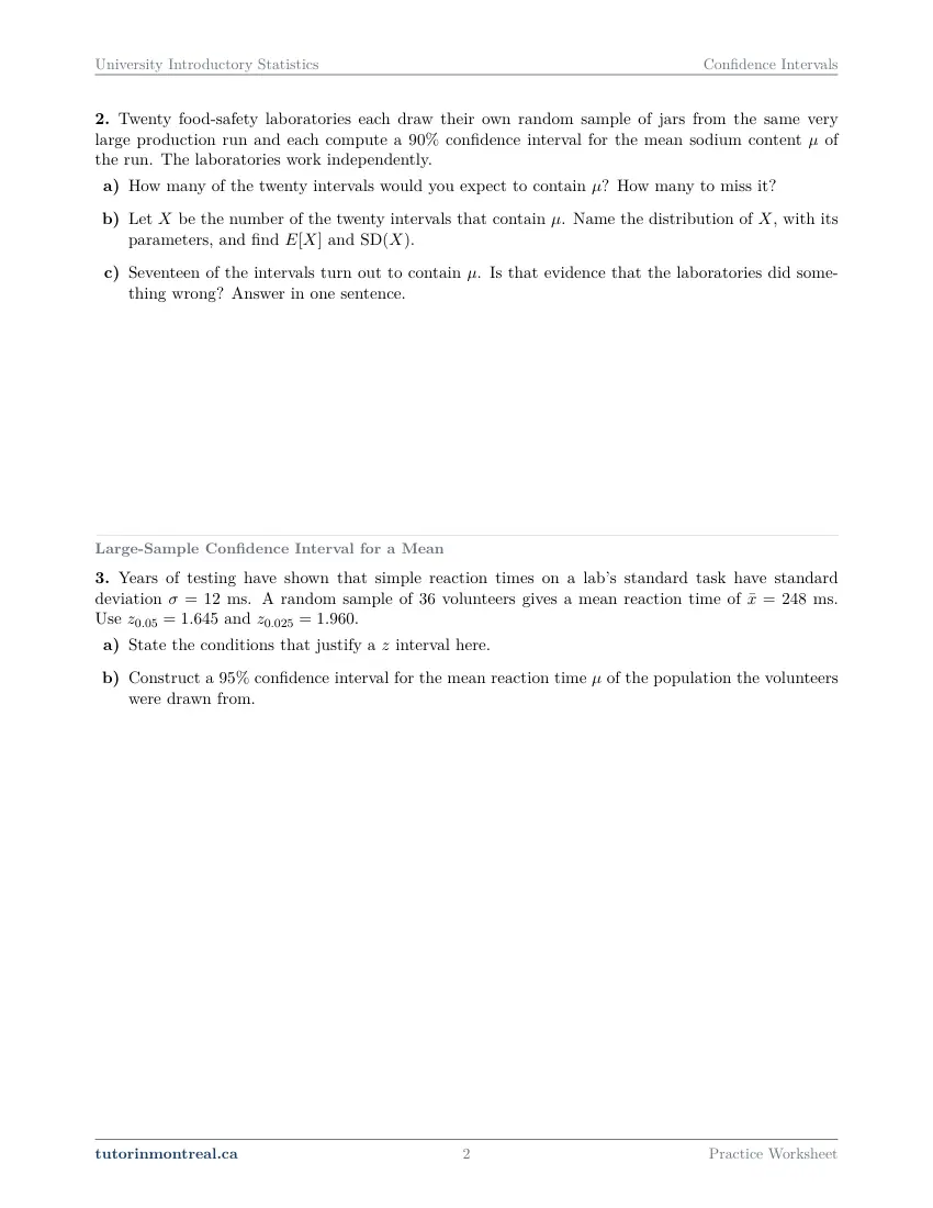
2. Q2Interpreting a Confidence Interval

   Twenty food-safety laboratories each draw their own random sample of jars from the same very large production run and each compute a $90\%$ confidence interval for the mean sodium content $\mu$ of the run. The laboratories work independently.

   1. How many of the twenty intervals would you expect to contain $\mu$? How many to miss it?
   2. Let $X$ be the number of the twenty intervals that contain $\mu$. Name the distribution of $X$, with its parameters, and find $E[X]$ and $SD(X)$.
   3. Seventeen of the intervals turn out to contain $\mu$. Is that evidence that the laboratories did something wrong? Answer in one sentence.
3. Q3Large-Sample Confidence Interval for a Mean

   Years of testing have shown that simple reaction times on a lab's standard task have standard deviation $\sigma =12$ ms. A random sample of $36$ volunteers gives a mean reaction time of $\overline{x}=248$ ms. Use $z_{0.05}=1.645$ and $z_{0.025}=1.960$.

   1. State the conditions that justify a $z$ interval here.
   2. Construct a $95\%$ confidence interval for the mean reaction time $\mu$ of the population the volunteers were drawn from.
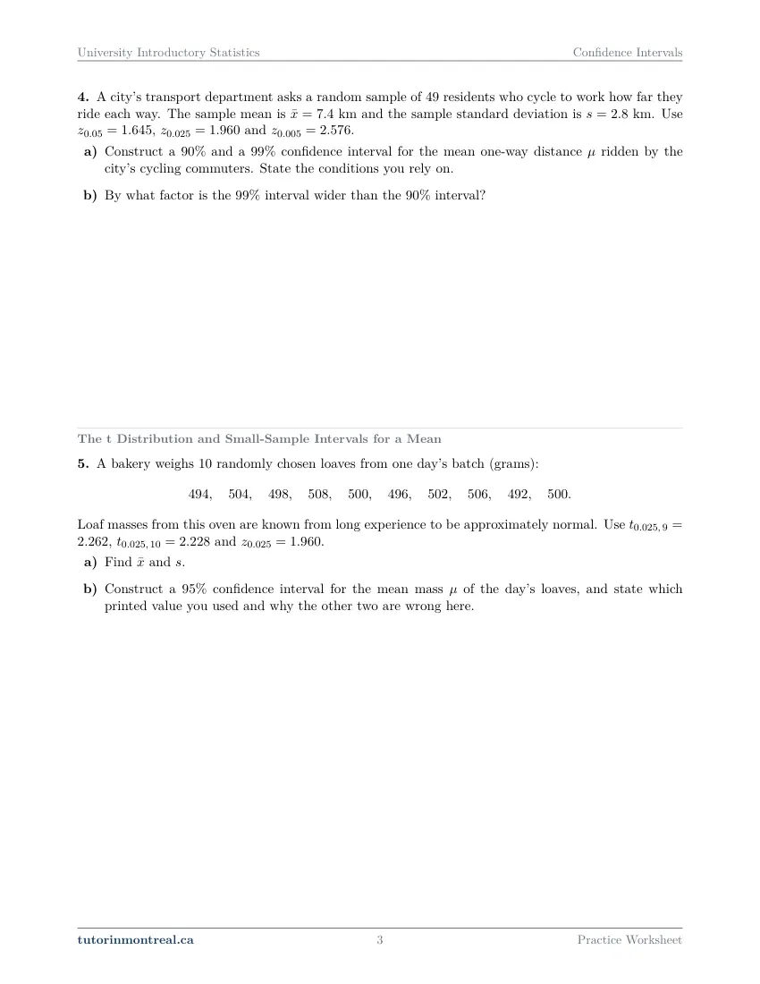
4. Q4Large-Sample Confidence Interval for a Mean

   A city's transport department asks a random sample of $49$ residents who cycle to work how far they ride each way. The sample mean is $\overline{x}=7.4$ km and the sample standard deviation is $s=2.8$ km. Use $z_{0.05}=1.645$, $z_{0.025}=1.960$ and $z_{0.005}=2.576$.

   1. Construct a $90\%$ and a $99\%$ confidence interval for the mean one-way distance $\mu$ ridden by the city's cycling commuters. State the conditions you rely on.
   2. By what factor is the $99\%$ interval wider than the $90\%$ interval?
5. Q5The t Distribution and Small-Sample Intervals for a Mean

   A bakery weighs $10$ randomly chosen loaves from one day's batch (grams): $$494,504,498,508,500,496,502,506,492,500.$$ Loaf masses from this oven are known from long experience to be approximately normal. Use $t_{0.025,9}=2.262$, $t_{0.025,10}=2.228$ and $z_{0.025}=1.960$.

   1. Find $\overline{x}$ and $s$.
   2. Construct a $95\%$ confidence interval for the mean mass $\mu$ of the day's loaves, and state which printed value you used and why the other two are wrong here.
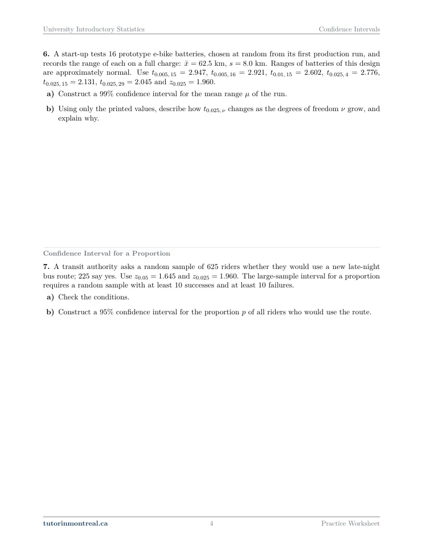
6. Q6The t Distribution and Small-Sample Intervals for a Mean

   A start-up tests $16$ prototype e-bike batteries, chosen at random from its first production run, and records the range of each on a full charge: $\overline{x}=62.5$ km, $s=8.0$ km. Ranges of batteries of this design are approximately normal. Use $t_{0.005,15}=2.947$, $t_{0.005,16}=2.921$, $t_{0.01,15}=2.602$, $t_{0.025,4}=2.776$, $t_{0.025,15}=2.131$, $t_{0.025,29}=2.045$ and $z_{0.025}=1.960$.

   1. Construct a $99\%$ confidence interval for the mean range $\mu$ of the run.
   2. Using only the printed values, describe how $t_{0.025,\nu }$ changes as the degrees of freedom $\nu$ grow, and explain why.
7. Q7Confidence Interval for a Proportion

   A transit authority asks a random sample of $625$ riders whether they would use a new late-night bus route; $225$ say yes. Use $z_{0.05}=1.645$ and $z_{0.025}=1.960$. The large-sample interval for a proportion requires a random sample with at least $10$ successes and at least $10$ failures.

   1. Check the conditions.
   2. Construct a $95\%$ confidence interval for the proportion $p$ of all riders who would use the route.
8. Q8Confidence Interval for a Proportion

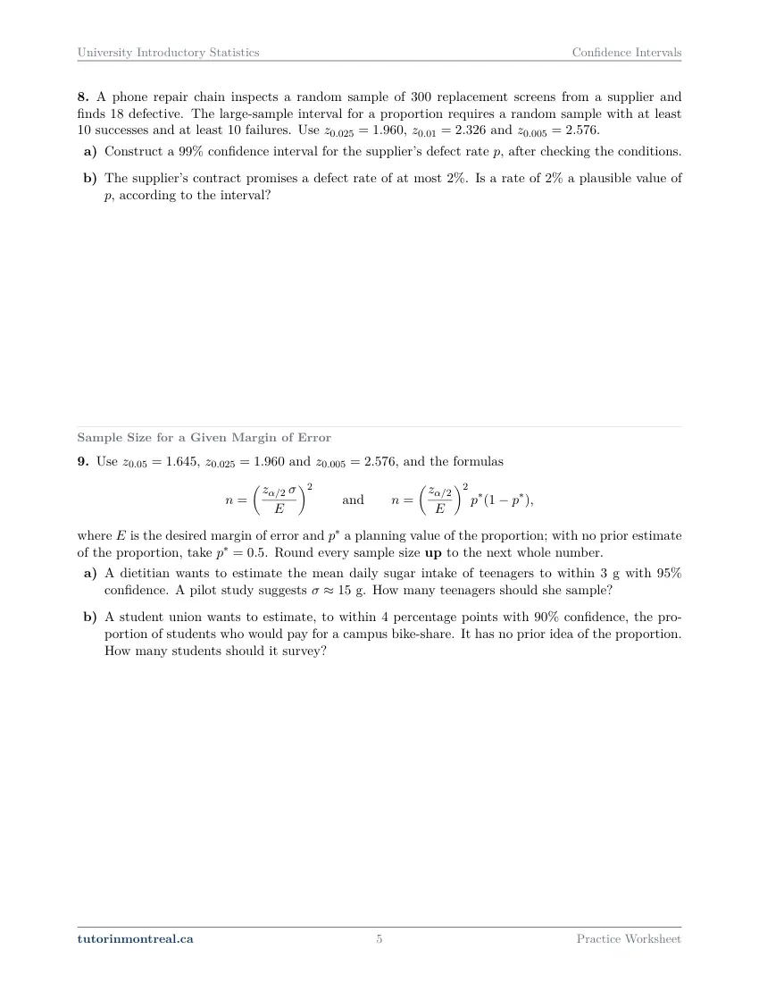
   A phone repair chain inspects a random sample of $300$ replacement screens from a supplier and finds $18$ defective. The large-sample interval for a proportion requires a random sample with at least $10$ successes and at least $10$ failures. Use $z_{0.025}=1.960$, $z_{0.01}=2.326$ and $z_{0.005}=2.576$.

   1. Construct a $99\%$ confidence interval for the supplier's defect rate $p$, after checking the conditions.
   2. The supplier's contract promises a defect rate of at most $2\%$. Is a rate of $2\%$ a plausible value of $p$, according to the interval?
9. Q9Sample Size for a Given Margin of Error

   Use $z_{0.05}=1.645$, $z_{0.025}=1.960$ and $z_{0.005}=2.576$, and the formulas $$n={\left(\frac{z_{\alpha /2}\sigma }{E}\right)}^2\text{and}n={\left(\frac{z_{\alpha /2}}{E}\right)}^2{p}^{*}(1-p^{*}),$$ where $E$ is the desired margin of error and $p^{*}$ a planning value of the proportion; with no prior estimate of the proportion, take $p^{*}=0.5$. Round every sample size up to the next whole number.

   1. A dietitian wants to estimate the mean daily sugar intake of teenagers to within $3$ g with $95\%$ confidence. A pilot study suggests $\sigma \approx 15$ g. How many teenagers should she sample?
   2. A student union wants to estimate, to within $4$ percentage points with $90\%$ confidence, the proportion of students who would pay for a campus bike-share. It has no prior idea of the proportion. How many students should it survey?
10. Q10Synthesis — drawing on several topics in this unit

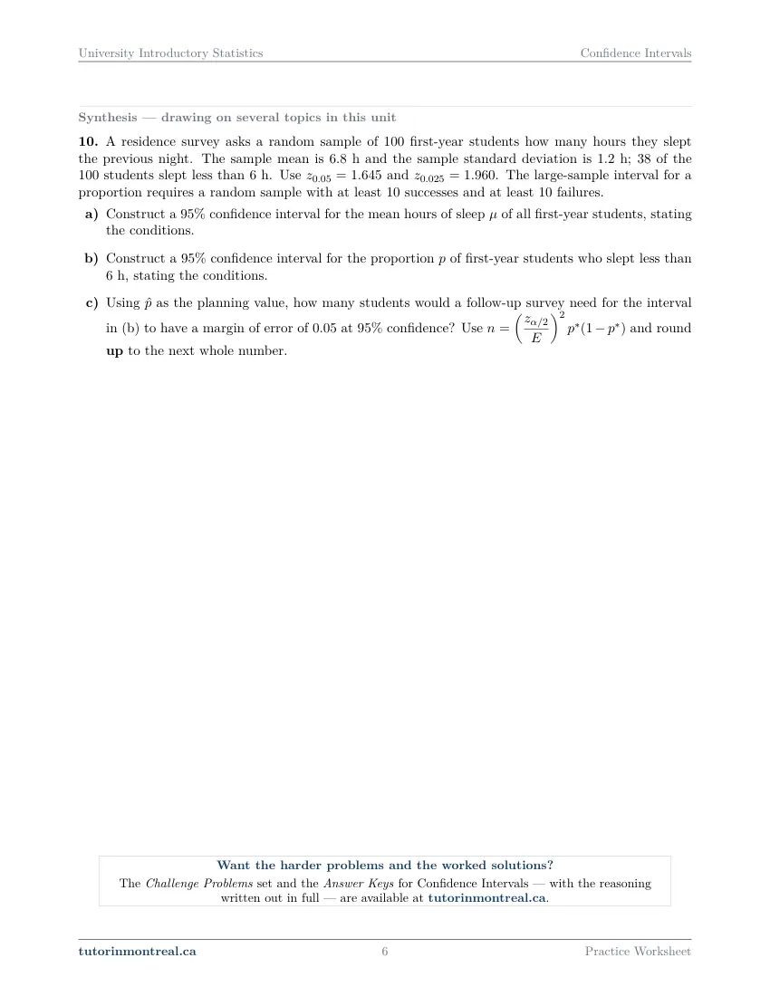
    A residence survey asks a random sample of $100$ first-year students how many hours they slept the previous night. The sample mean is $6.8$ h and the sample standard deviation is $1.2$ h; $38$ of the $100$ students slept less than $6$ h. Use $z_{0.05}=1.645$ and $z_{0.025}=1.960$. The large-sample interval for a proportion requires a random sample with at least $10$ successes and at least $10$ failures.

    1. Construct a $95\%$ confidence interval for the mean hours of sleep $\mu$ of all first-year students, stating the conditions.
    2. Construct a $95\%$ confidence interval for the proportion $p$ of first-year students who slept less than $6$ h, stating the conditions.
    3. Using $\widehat{p}$ as the planning value, how many students would a follow-up survey need for the interval in (b) to have a margin of error of $0.05$ at $95\%$ confidence? Use $n={\left({\displaystyle \frac{z_{\alpha /2}}{E}}\right)}^2{p}^{*}(1-p^{*})$ and round up to the next whole number.

The 7 challenge problems for this topic are a separate, paid sheet and are not reproduced here.

How to do every concept on this sheet

This is the part worksheet sites usually leave out. Below is the actual reasoning behind each group of questions — not a full solution set, the decisions that get you to one. Read it before you start, or after you get stuck.

Every interval on this sheet has the same three parts

Before the topics separate, notice what they share. An interval is an estimate, a critical value and a standard error, assembled the same way every time:

The estimate is x̄ for a mean and p̂ for a proportion. The critical value comes from the confidence level, through the tail area α/2. The standard error is σ/√n, s/√n or √(p̂(1 − p̂)/n) depending on which parameter is being estimated and what is known about the population. The product of the last two is the margin of error, and the whole width of the interval is twice it. Almost every question below is one of these three slots being filled, checked, or read backwards.

What a confidence level actually says

A confidence level is a property of the procedure, not of the one interval in front of you. Repeat the whole experiment — new random sample, same method — and a 90 per cent procedure produces intervals that capture the parameter 90 per cent of the time in the long run. The parameter does not move; the interval does.

Q2 is that idea made concrete: twenty laboratories, twenty independent samples from the same production run, twenty intervals at the same level. Q2(a) asks how many of them would be expected to contain μ and how many to miss it, and the only thing you need is the long-run proportion applied to twenty repetitions. Q2(b) then turns the count of hits into a random variable: ask whether the twenty laboratories are independent trials, whether each one has the same probability of a hit, and what counts as a success — those three answers name the distribution and its parameters, and its mean and standard deviation follow from the formulas already met in Discrete Random Variables.

Reading an interval backwards

Q1 gives you the finished interval and asks for the ingredients, which is the fastest way to prove you know how one is built. The interval is symmetric about the estimate, so the centre and the half-width are the two numbers you can read off any interval at sight:

That is Q1(a). Q1(b) then unpicks the margin of error itself: it was built as a critical value times s/√n, and everything in that product except s is either printed in the question or already found, so one line of algebra returns s. Work in the order the formula was assembled, and substitute the critical value that belongs to the level the interval was actually reported at — not the one you would have used.

The large-sample z interval for a mean

Q3 is the cleanest case there is: a standard deviation established outside this sample, over years of testing, and a sample large enough for the central limit theorem to apply.

Q3(a) asks for the conditions before the interval, and they are worth writing as a list rather than a sentence, because each one is checkable and each one can fail on its own.

Q3(b) is then the formula, with one caution: keep the units the question uses all the way through, and give the answer as an interval with both endpoints and the units attached, not as a lone margin of error.

Q4 is the large-sample interval in its more common form — no σ anywhere, only s from the sample — and it asks for two levels from one set of data. Build them as one calculation: the standard error is computed once, and the two intervals differ only in the critical value multiplying it. Q4(a) also asks for the conditions, and here condition 2 above is the one that needs a sentence: say explicitly that s is standing in for σ and that the sample size is what makes that acceptable.

The t distribution and small samples

When σ is unknown and the sample is small, s/√n is not a reliable stand-in for the true standard error, and the extra uncertainty has to be paid for. The t distribution is the price: same symmetric bell shape, heavier tails, and a shape that depends on one number.

Q5 starts from raw data: ten loaf masses, from which Q5(a) wants x̄ and s by hand. Two habits make that reliable. Subtract a convenient round number from every value first — the standard deviation is unchanged by a shift, and the arithmetic becomes small whole numbers — and keep the sum of squared deviations unrounded until the very end, because rounding s early moves both endpoints. The question also tells you the masses are approximately normal, which is the condition that licenses a t interval at a sample size this small; say so.

Q6 gives x̄ and s ready-made and tests the choice of critical value instead, with seven printed values to choose between. Q6(a) is the interval; the tail area comes from the confidence level and the degrees of freedom from the sample size, and together they pick exactly one of the seven. Q6(b) then asks you to read a pattern off the printed list: line up only the values that share a tail area, put them in order of their degrees of freedom, describe how they move, and explain the movement from what t is for. The explanation is the marked part — connect the behaviour to how much uncertainty is left in s as the sample grows, and to the standard normal value sitting at the end of the list.

Intervals for a proportion

A proportion is a mean of zeros and ones, so the interval has the same three parts; only the standard error changes, and the estimate replaces the unknown p inside it.

Q7 and Q8 both state the condition in the question itself — a random sample with at least ten successes and at least ten failures — and both ask you to check it rather than assume it. Checking it means counting the successes and the failures in this sample and comparing each with ten, in writing. The condition is what lets a normal critical value be used on a count that is not normal; when it fails, this interval is simply not available and no adjustment on this sheet repairs it.

Q8(b) is the interpretation question, and it is the one that carries the marks. A confidence interval is a set of plausible values for p: a value inside it is consistent with the data at that level, and a value outside it is not. So the work is to compare the promised rate with the two endpoints and say which side of them it falls on — then answer in a sentence about the supplier's rate, not about the arithmetic. Be careful to compare like with like: a rate quoted in percentage points has to be written as a proportion, or both endpoints converted, before any comparison is meaningful.

Sample size for a given margin of error

Q9 runs the whole calculation backwards. The margin of error is chosen first, and the question is what n delivers it. Both formulas are printed in the question; the work is in reading which one applies and in supplying the planning value each needs.

Q9(a) is the mean case with σ supplied by a pilot study, and Q9(b) the proportion case with nothing known in advance. Note in passing what the formulas say about the cost of precision: halving E multiplies n by four, because E sits squared in the denominator. That relationship is worth stating in a sentence whenever a question asks why a small margin of error is expensive.

The synthesis question

Q10 takes one survey and asks three different things of it, which is the exam-shaped version of this whole set. The same hundred students yield a mean in Q10(a) and a proportion in Q10(b), so the first decision each time is which parameter the question is about, and therefore which standard error and which condition apply. Both parts ask for the conditions explicitly: the mean needs the random sample and a sample size large enough for the central limit theorem; the proportion needs the random sample and the success-and-failure counts, which here have to be read out of the survey description rather than handed to you.

Q10(c) closes the loop back to Q9. A follow-up survey is being planned, the margin of error is specified in advance, and the planning value is no longer a guess — it is the p̂ this survey produced. Use the printed formula, keep E as a proportion, and round up. Then read your answer against the hundred students already surveyed: a sample-size calculation that returns a number smaller than the one you have is usually a sign that E was entered in percentage points.

Preview all 6 pages

Click any page to open the full PDF.

Getting the most out of it

Write the three slots before you compute anything

Estimate, critical value, standard error — set them out as three labelled lines, then fill them. It makes the z-versus-t decision and the mean-versus-proportion decision visible instead of implicit, and a question that supplies a list of critical values is usually testing exactly those two decisions.

Name the population out loud

Trout in one lake, volunteers at one laboratory, riders of one transit system, first-year students in one residence: the interval is about the population the sample came from and no other. Saying it before you start is what keeps the final sentence honest and stops a result about one group being reported as a result about everyone.

Predict the direction before you recompute

Raise the confidence level, or shrink the sample: does the interval get wider or narrower? The formula answers both in a second, because only one factor moves. Predicting first and checking after turns every recomputation into a free error check, and it is what questions like Q1(c) and Q4(b) are training.

Keep the intermediate values unrounded

Round s, then the standard error, then the margin of error, and the endpoints can drift enough to change an interpretation. Carry full precision through the calculator and round once, at the endpoints, to the precision the data justify.

Re-read the condition list after each answer

Random sample; σ known or estimated; normal population or large n; at least ten successes and ten failures. Most of the marks that go missing on this topic are not arithmetic — they are a condition that was true and never written down, or false and never noticed.

Common questions