University Business Mathematics — Curve Analysis and Business Optimization Worksheet

All 11 questions

Each question targets one named concept from the sheet. Read them here, or print the PDF — it has working space under each one.

1. Q1The First Derivative, Critical Numbers and Local Extrema

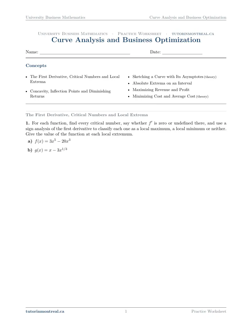
   For each function, find every critical number, say whether $f^{\prime }$ is zero or undefined there, and use a sign analysis of the first derivative to classify each one as a local maximum, a local minimum or neither. Give the value of the function at each local extremum.

   1. $f(x)=3x^5-20x^3$
   2. $g(x)=x-3x^{1/3}$
2. Q2The First Derivative, Critical Numbers and Local Extrema

   A tutoring agency opens a new branch. The number of students enrolled $t$ months after opening is modelled by $$N(t)=t^3-18t^2+81t+40,0\le t\le 12.$$

   1. On which time intervals is enrolment rising, and on which is it falling?
   2. Find each local maximum and local minimum of enrolment, with the month at which it occurs, and describe in one sentence what happens to enrolment over the year.
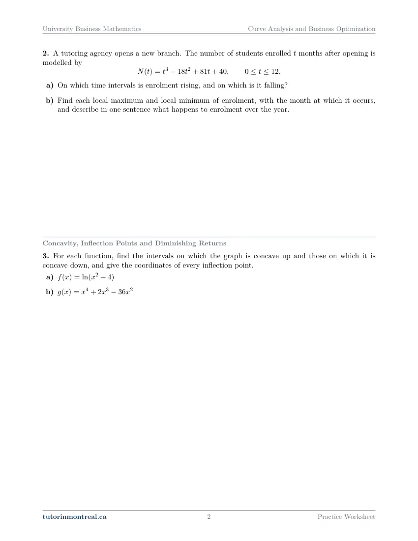
3. Q3Concavity, Inflection Points and Diminishing Returns

   For each function, find the intervals on which the graph is concave up and those on which it is concave down, and give the coordinates of every inflection point.

   1. $f(x)=\ln (x^2+4)$
   2. $g(x)=x^4+2x^3-36x^2$
4. Q4Concavity, Inflection Points and Diminishing Returns

   A regional furniture retailer finds that its monthly revenue $R$, in thousands of dollars, depends on its monthly advertising budget $x$, in thousands of dollars: $$R(x)=-x^3+36x^2+50x+300,0\le x\le 20.$$

   1. Show that revenue increases with the advertising budget over the whole range.
   2. Find the point of diminishing returns: the budget at which the rate of increase of revenue is greatest. Give the revenue and the value of $R^{\prime }$ there, with units.
   3. Compute $R^{\prime }(8)$ and $R^{\prime }(16)$ and say in one sentence what the comparison tells the retailer.
5. Q5Sketching a Curve with Its Asymptotes

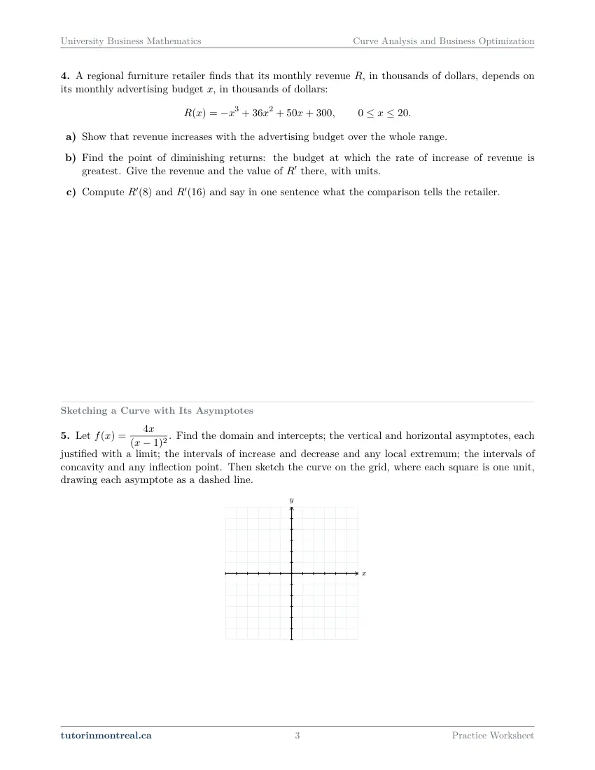
   Let $f(x)={\displaystyle \frac{4x}{(x-1{)}^2}}$. Find the domain and intercepts; the vertical and horizontal asymptotes, each justified with a limit; the intervals of increase and decrease and any local extremum; the intervals of concavity and any inflection point. Then sketch the curve on the grid, where each square is one unit, drawing each asymptote as a dashed line.

   A blank Cartesian grid for this question is on the printable PDF.

6. Q6Absolute Extrema on an Interval

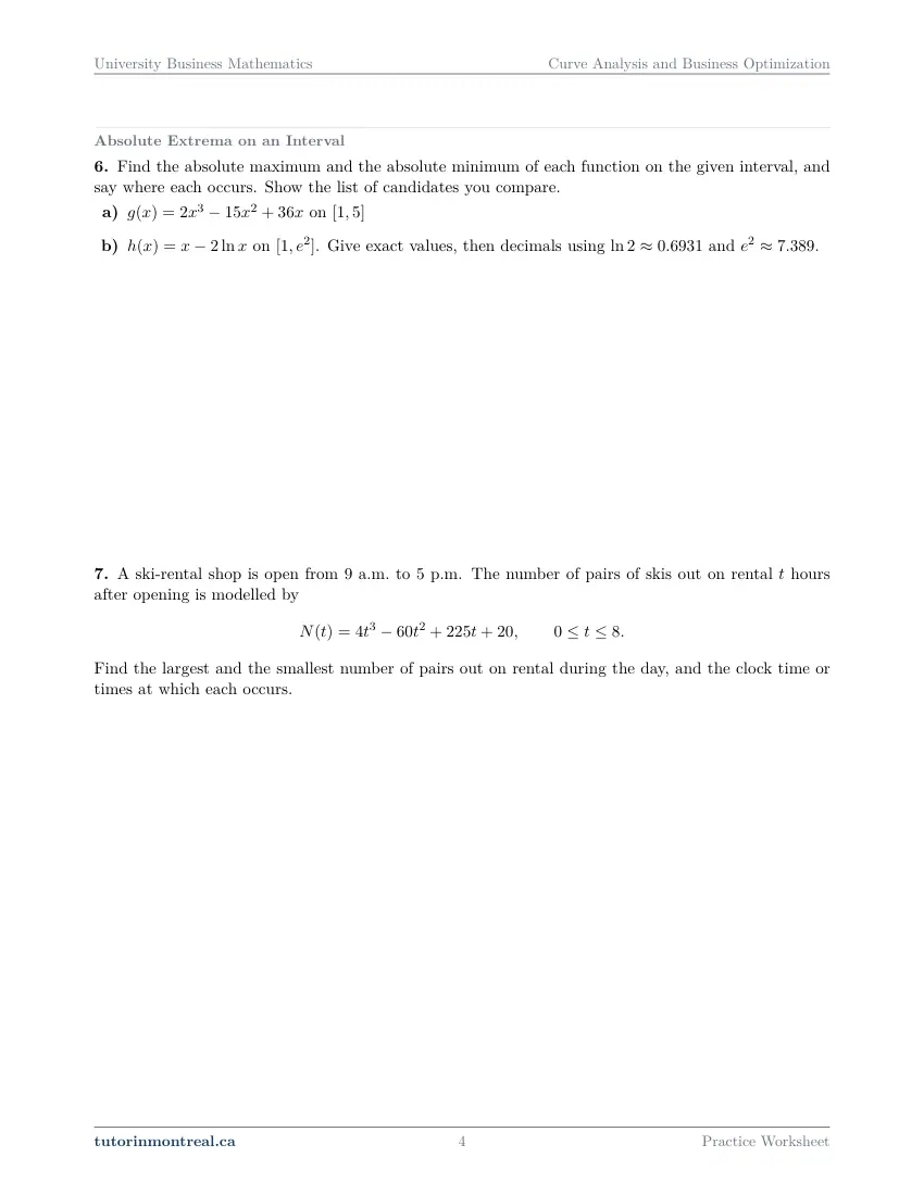
   Find the absolute maximum and the absolute minimum of each function on the given interval, and say where each occurs. Show the list of candidates you compare.

   1. $g(x)=2x^3-15x^2+36x$ on $[1,5]$
   2. $h(x)=x-2\ln x$ on $[1,e^2]$. Give exact values, then decimals using $\ln 2\approx 0.6931$ and $e^2\approx 7.389$.
7. Q7Absolute Extrema on an Interval

   A ski-rental shop is open from 9 a.m. to 5 p.m. The number of pairs of skis out on rental $t$ hours after opening is modelled by $$N(t)=4t^3-60t^2+225t+20,0\le t\le 8.$$ Find the largest and the smallest number of pairs out on rental during the day, and the clock time or times at which each occurs.

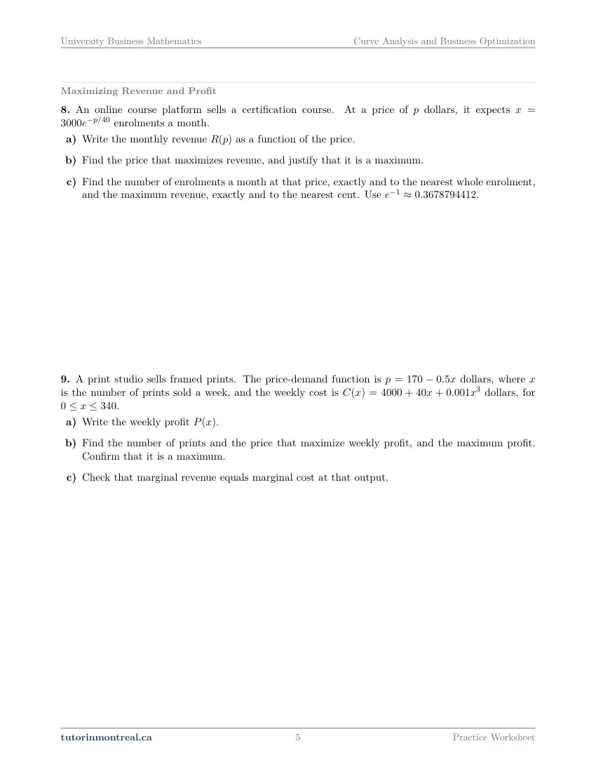
8. Q8Maximizing Revenue and Profit

   An online course platform sells a certification course. At a price of $p$ dollars, it expects $x=3000e^{-p/40}$ enrolments a month.

   1. Write the monthly revenue $R(p)$ as a function of the price.
   2. Find the price that maximizes revenue, and justify that it is a maximum.
   3. Find the number of enrolments a month at that price, exactly and to the nearest whole enrolment, and the maximum revenue, exactly and to the nearest cent. Use $e^{-1}\approx 0.3678794412$.
9. Q9Maximizing Revenue and Profit

   A print studio sells framed prints. The price-demand function is $p=170-0.5x$ dollars, where $x$ is the number of prints sold a week, and the weekly cost is $C(x)=4000+40x+0.001x^3$ dollars, for $0\le x\le 340$.

   1. Write the weekly profit $P(x)$.
   2. Find the number of prints and the price that maximize weekly profit, and the maximum profit. Confirm that it is a maximum.
   3. Check that marginal revenue equals marginal cost at that output.
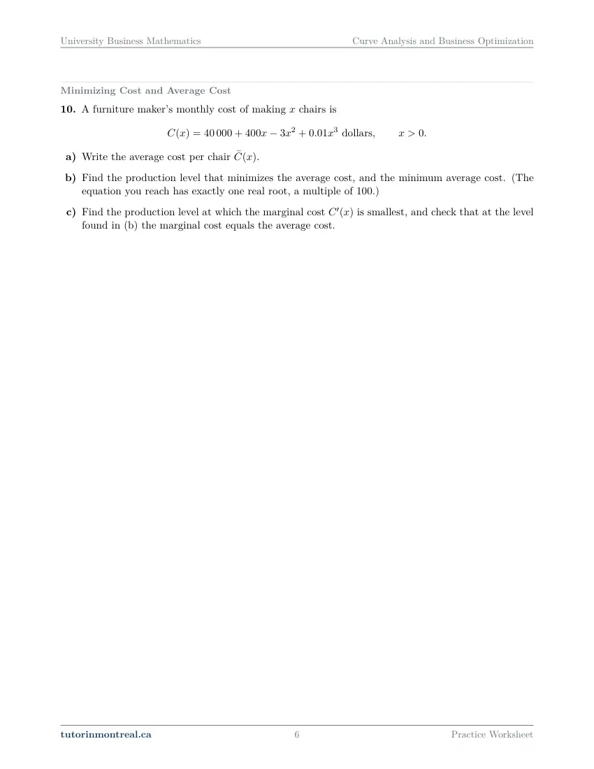
10. Q10Minimizing Cost and Average Cost

    A furniture maker's monthly cost of making $x$ chairs is $$C(x)=40000+400x-3x^2+0.01x^3\text{dollars},x>0.$$

    1. Write the average cost per chair $\overline{C}(x)$.
    2. Find the production level that minimizes the average cost, and the minimum average cost. (The equation you reach has exactly one real root, a multiple of $100$.)
    3. Find the production level at which the marginal cost $C^{\prime }(x)$ is smallest, and check that at the level found in (b) the marginal cost equals the average cost.
11. Q11Synthesis — drawing on several topics in this unit

    A small electronics assembler's weekly profit, in dollars, from $x$ hundred units is $$P(x)=-x^3+75x^2-675x-5000,0\le x\le 60,$$ where $60$ hundred units is the plant's weekly capacity.

    1. Find the intervals on which profit increases and decreases, and classify each critical number.
    2. Find the inflection point and explain what it means for the marginal profit.
    3. Find the absolute maximum and minimum profit on $[0,60]$, and the output at each.

The 7 challenge problems for this topic are a separate, paid sheet and are not reproduced here.

How to do every concept on this sheet

This is the part worksheet sites usually leave out. Below is the actual reasoning behind each group of questions — not a full solution set, the decisions that get you to one. Read it before you start, or after you get stuck.

Critical numbers and the first-derivative test

A critical number of f is a number c in the domain of f where f′(c) = 0 or f′(c) does not exist. Those are the only places a local maximum or minimum can occur, but not every critical number is one. The first-derivative test decides: watch the sign of f′ as x passes through c.

Q1 asks for exactly this, and also for which kind of critical number each one is — zero or undefined. In Q1(a) the derivative is a polynomial, so it exists everywhere; factor out the highest common power of x before you solve. In Q1(b) the exponent 1/3 changes the picture: the power rule produces a negative fractional power, so rewrite the derivative as a single fraction with a cube root in it, then examine the numerator and the denominator separately — one tells you where f′ is zero, the other where it fails to exist.

Q2 puts the same test into a model: enrolment N(t) at a tutoring agency over its first twelve months. "Rising" and "falling" are the intervals where N′ is positive and negative, and the domain 0 ≤ t ≤ 12 is where the chart starts and stops. The one-sentence summary in Q2(b) is the sign chart read aloud in the language of the business, with the month at which each turn happens.

Concavity, inflection points and diminishing returns

The second derivative does for the slope what the first does for the function. Where f″ > 0 the graph is concave up and f′ is increasing; where f″ < 0 it is concave down and f′ is decreasing. An inflection point is a point on the graph where the concavity actually changes — so it needs a sign chart of f″, built exactly like the one for f′.

Q3(a) is a chain-rule function: the derivative of ln(x² + 4) is a quotient, so the second derivative needs the quotient rule, and it is worth simplifying the numerator fully before you look for its zeros. Note that x² + 4 is never zero, so the domain is every real number. Q3(b) is a quartic whose second derivative is a quadratic; factor it and chart it. In both parts, give each inflection point as a pair of coordinates, which means evaluating f, not f″.

Q4 is built on that idea. Part (a) asks you to show that R′ stays positive over the whole range of budgets: find the smallest value R′ takes on the closed interval, which is a small absolute-extremum problem in its own right. Part (b) is the inflection point of R, reported with its units — the budget and the revenue in thousands of dollars, and R′ in thousands of dollars of revenue per thousand dollars of advertising. Part (c) compares two marginal values and asks what the comparison means for the retailer; say it in terms of what the next thousand dollars of advertising returns.

Sketching a curve with its asymptotes

Q5 puts every tool of the unit on one rational function. Do the parts in a fixed order, and collect the results in a single table before you draw anything.

Absolute extrema on a closed interval

A continuous function on a closed interval [a, b] always has an absolute maximum and an absolute minimum, and they can only occur at a critical number inside the interval or at an endpoint. So the method is a list and a comparison, with no sign chart needed.

Q6 asks you to show the list, which is the whole of the method's justification. In Q6(a), check each critical number against the interval before you evaluate — a critical number outside [1, 5] is not a candidate. In Q6(b), the function mixes x and ln x on [1, e²]: find the critical number from h′, check that it lies in the interval, and give each value exactly first, with ln written as ln, before turning it into a decimal with the approximations supplied.

Q7 is the same method in a model: skis out on rental over an eight-hour day. Two things are specific to it. The "largest and smallest number of pairs" are values of N, not values of t. And t counts hours after opening at 9 a.m., so every t you find has to be translated into a clock time — and the question allows for a value to be reached at more than one time, so look at your list for ties before you answer.

Maximizing revenue and profit

Every revenue and profit problem in this course follows the same chain, and most errors come from skipping a link in it.

Q8 gives demand as a function of price, so revenue is naturally a function of p: multiply the price by the exponential demand and use the product rule. The factor e^(−p/40) is never zero, which is what makes the equation R′(p) = 0 short. Part (c) asks for the enrolments and the revenue at the optimal price, each exactly and then rounded, using the value of e^(−1) provided.

Q9 gives the opposite arrangement: price as a function of quantity, p = 170 − 0.5x. Now revenue is a function of x, profit is R(x) − C(x), and the cubic term in the cost makes P′(x) = 0 a quadratic. Only a root inside 0 ≤ x ≤ 340 counts. Part (b) wants three things — the number of prints, the price at that number (from the demand equation, not from the profit), and the maximum profit — and a confirmation. Part (c) is the check every economist makes.

Minimizing cost and average cost

Total cost almost always increases with output, so "minimize cost" in a business course means minimize the cost per unit. The average cost is the total divided by the number of units.

In Q10, divide each term of C(x) by x before differentiating: the fixed cost becomes a term in 1/x and the rest become simple powers, so C̄′ needs only the power rule. Clearing the denominator in C̄′(x) = 0 leaves a cubic; the question tells you something about its one real root, which is your cue to test multiples of 100 and then factor. Justify the minimum with the sign of C̄′ on either side, or with C̄″.

Q10(c) asks for two different things, and they are easy to confuse. The level where the marginal cost C′(x) is smallest is found from C″(x) = 0 — it is an inflection point of the total cost, the same idea as Q4's point of diminishing returns. The second half is a check, not a new calculation: evaluate C′ and C̄ at your answer to part (b) and compare.

The synthesis question

Q11 runs the whole unit on one profit function, with output in hundreds of units and a capacity of sixty hundred. Part (a) is Q1 and Q2: factor P′, chart it on [0, 60] and classify each critical number. Part (b) is Q4's idea applied to profit — the inflection point of P is where the marginal profit P′ reaches an extreme value, and the explanation should say whether that is its largest or its smallest value and what that means for the next hundred units. Part (c) is Q6 and Q7: the critical numbers and both ends of the capacity interval go on one list, and you report each extreme profit together with the output that produces it.

Preview all 7 pages

Click any page to open the full PDF.

Getting the most out of it

Factor before you chart

Every question in this set ends in a sign chart, and a sign chart can only be read from a factored derivative. Spend the extra line factoring out common powers and constants; it is faster than testing an unfactored polynomial at every test value.

Keep f, f′ and f″ in separate columns

Extrema come from f′, inflection points from f″, and every coordinate you report comes from f. Most lost marks in this unit are a y-value read off the wrong function, so label each row of your table with the function it came from.

Write the candidates list every time

For an absolute extremum, list the critical numbers inside the interval and both endpoints, with the value of the function at each, before you name a winner. The list is the justification; without it, the answer is a guess that happens to be right.

Finish with units and a sentence

A business optimization is answered when a manager could act on it: the quantity, the price, the value achieved, each with its unit, and one sentence in words. Check that the answer lies in the domain the model allows.

Common questions