University Business Mathematics — Linear Inequalities and Linear Programming Worksheet
How a business with limited hours, space and materials decides what to make. The set starts with one inequality and its half-plane, builds up to a system and the feasible region it cuts out, finds the corner points of regions that close up and regions that run off the grid, and then turns word problems — a skate shop, a feed mill, a cider mill, a fertilizer purchase — into linear programming models and solves them on a graph. Every question is set in a business context, and every one asks you to say what the mathematics means for the decision. Have a look on this page, then print the free PDF when you want to write on it.
Practice worksheet — free PDF
No email, no account, no watermark. Teachers: photocopy it for your classes freely. Worked solutions and 6 harder problems come with the University Business Math bundle.
2 of the 9 questions
Each question targets one named concept from the sheet. Read them here, or print the PDF — it has working space under each one. 2 of the 9 questions are printed below. The other 7 are built on a diagram or a table of values that does not translate to the page, so they are in the free PDF — marked below where they would have come.
-
Q1Graphing a Linear Inequality in Two Variables
This question is built around a diagram or a table of values. Open it in the PDF.
-
Q2Systems of Linear Inequalities and the Feasible Region
This question is built around a diagram or a table of values. Open it in the PDF.
-
Q3Systems of Linear Inequalities and the Feasible Region
This question is built around a diagram or a table of values. Open it in the PDF.
-
Q4Corner Points of Bounded and Unbounded Regions
This question is built around a diagram or a table of values. Open it in the PDF.
-
Q5Formulating a Linear Programming Model
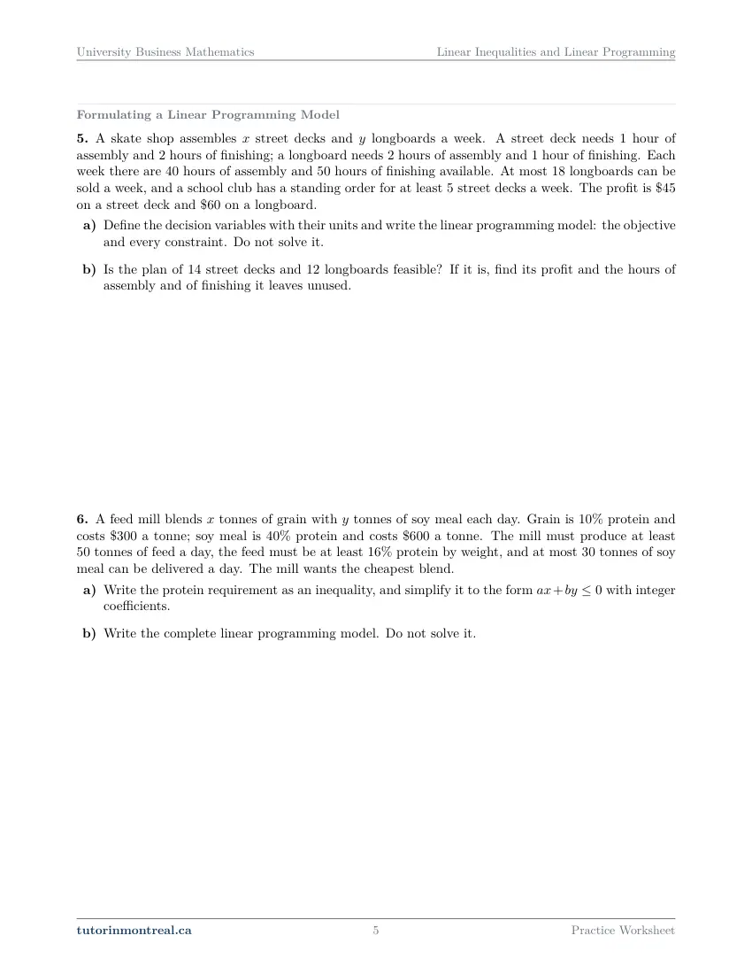
A skate shop assembles street decks and longboards a week. A street deck needs hour of assembly and hours of finishing; a longboard needs hours of assembly and hour of finishing. Each week there are hours of assembly and hours of finishing available. At most longboards can be sold a week, and a school club has a standing order for at least street decks a week. The profit is $45 on a street deck and $60 on a longboard.
- Define the decision variables with their units and write the linear programming model: the objective and every constraint. Do not solve it.
- Is the plan of street decks and longboards feasible? If it is, find its profit and the hours of assembly and of finishing it leaves unused.
-
Q6Formulating a Linear Programming Model
A feed mill blends tonnes of grain with tonnes of soy meal each day. Grain is protein and costs $300 a tonne; soy meal is protein and costs $600 a tonne. The mill must produce at least tonnes of feed a day, the feed must be at least protein by weight, and at most tonnes of soy meal can be delivered a day. The mill wants the cheapest blend.
- Write the protein requirement as an inequality, and simplify it to the form with integer coefficients.
- Write the complete linear programming model. Do not solve it.
-
Q7Solving a Linear Program Graphically
This question is built around a diagram or a table of values. Open it in the PDF.
-
Q8Solving a Linear Program Graphically
This question is built around a diagram or a table of values. Open it in the PDF.
-
Q9Synthesis — drawing on several topics in this unit
This question is built around a diagram or a table of values. Open it in the PDF.
The 6 challenge problems for this topic are a separate, paid sheet and are not reproduced here.
What does this set assume? This set assumes Secondary 5 mathematics only: graphing a line from its intercepts, solving a system of two linear equations by substitution or elimination, and the rule that multiplying an inequality by a negative number reverses it. It leans on the earlier University Business Mathematics sets only for their habits — reading a business story into variables, as in Functions for Business Models — and uses no calculus, so it sits comfortably before Limits, Derivatives and Marginal Analysis. Linear programming here is graphical and in two variables: formulate, draw the feasible region, test the corner points, and recognise an unbounded region. The simplex method and tableaux, duality and sensitivity analysis are deliberately not part of this set or this course.
Which course is this for? In the public course calendars of Montreal universities, this material is part of the courses numbered MATH 123, MATH 208, MATH 10601 and MAT1002. Each course orders and weights the topics its own way, so check your own outline for what your exam covers. Which sets match your course.
How to do every concept on this sheet
This is the part worksheet sites usually leave out. Below is the actual reasoning behind each group of questions — not a full solution set, the decisions that get you to one. Read it before you start, or after you get stuck.
One inequality, one half-plane
A linear inequality in x and y is satisfied by every point on one side of a line. The line itself is the boundary, and the whole method is three decisions: where the line is, whether it belongs to the solution set, and which side to shade.
Graphing ax + by ≤ c
Three decisions, in this order.
- 1Draw the boundary
Replace the inequality sign by = and find the two intercepts: set x = 0 to get the y-intercept, then y = 0 to get the x-intercept. Two points fix the line.
- 2Solid or dashed
≤ and ≥ include the line, so draw it solid. < and > exclude it, so draw it dashed.
- 3Pick a side with a test point
Substitute a point not on the line — the origin, whenever the line misses it. If the point satisfies the inequality, shade its side; if not, shade the other.
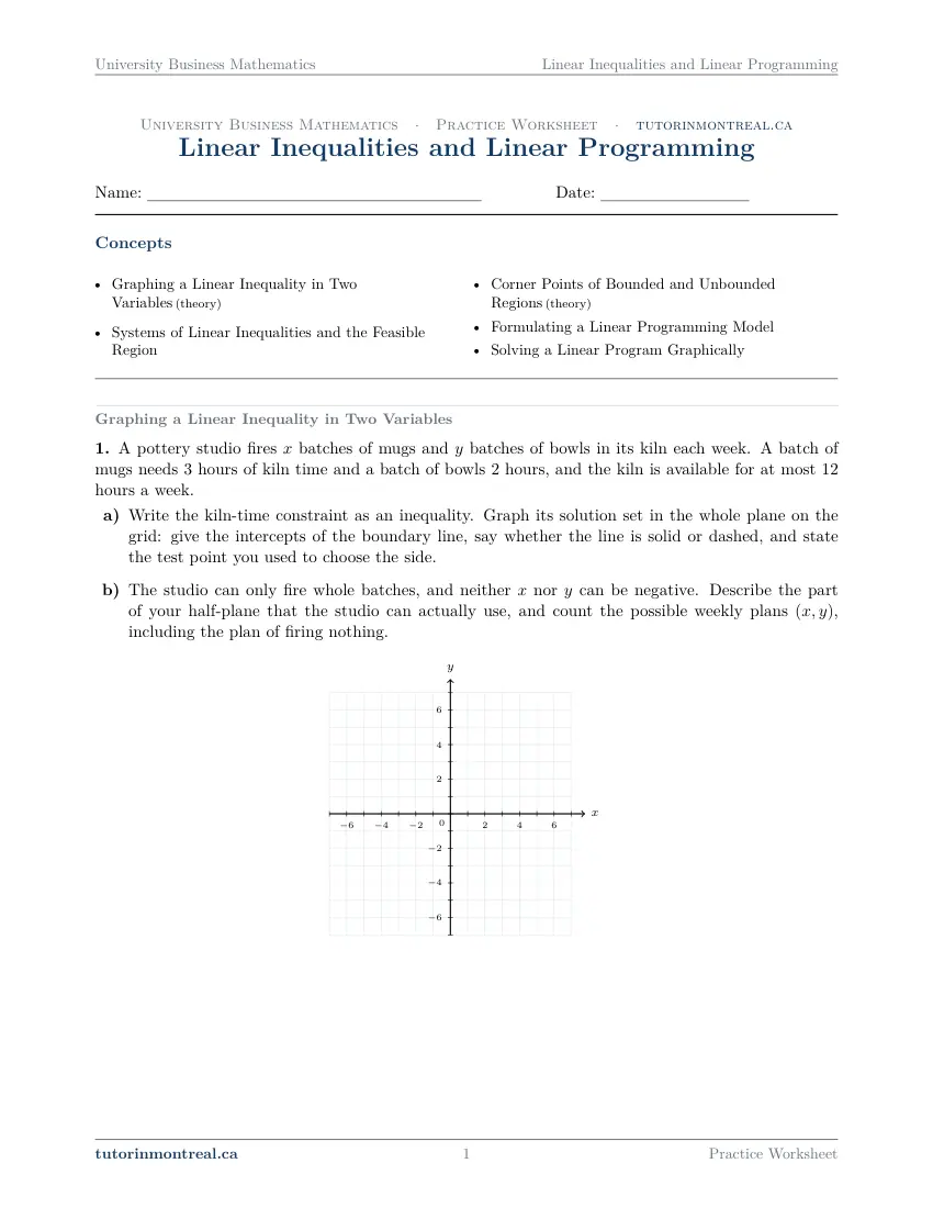
Q1(a) asks for all three decisions in writing, and on the whole plane, before any business restriction applies. Q1(b) then adds what the story imposes: batches cannot be negative, and they come in whole numbers. The usable part is no longer a shaded region but a set of lattice points inside it, and counting them is a matter of going column by column — for each whole value of x, which whole values of y still fit.
A test point never lies on the line. If the boundary passes through the origin, the origin tells you nothing; use a point such as (1, 0) or (0, 1) instead.
Systems of inequalities and the feasible region
Each constraint shades a half-plane; the feasible region is the set of points that lie in every one of them at once. In a business problem, the constraints almost always include x ≥ 0 and y ≥ 0, which confine everything to the first quadrant. Write those two down every time — a model without them is incomplete, even when the story never mentions them.
Shade the rejected side. With four or five constraints, shading each accepted half-plane turns the grid into a smudge. Many students hatch the side each constraint rejects instead, so that the feasible region is the one area left clean.
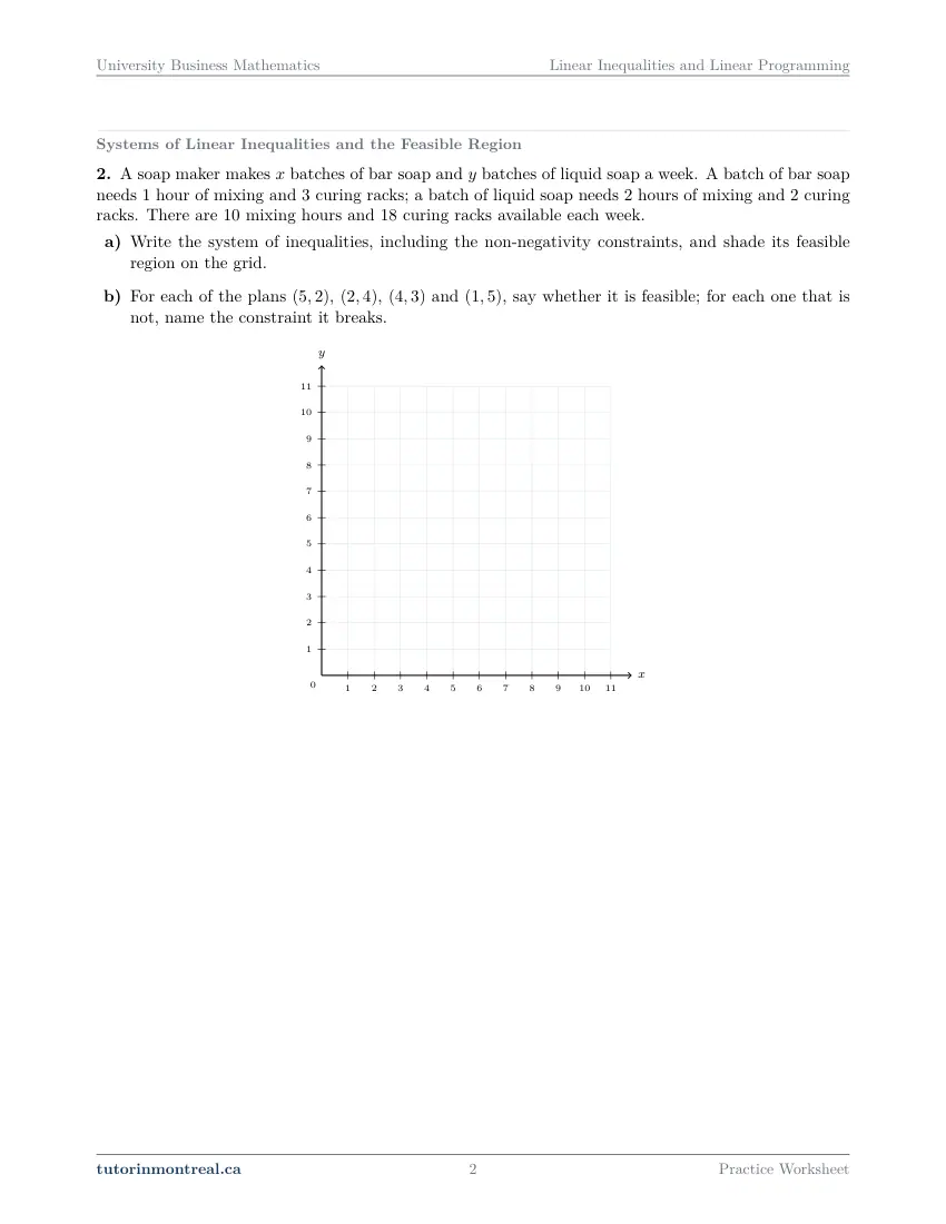
Q2 builds a system from a resource table: one inequality for mixing hours and one for curing racks, each saying that what a plan uses cannot exceed what is available, plus the two non-negativity constraints. Q2(b) asks you to test four plans. Substitute each plan into every constraint in turn; a plan is feasible only if it passes all of them, and when it fails, the question wants the name of the constraint it breaks, not just a verdict. A plan that breaks one constraint may well satisfy the other, and saying which one is what tells the manager what is in short supply.
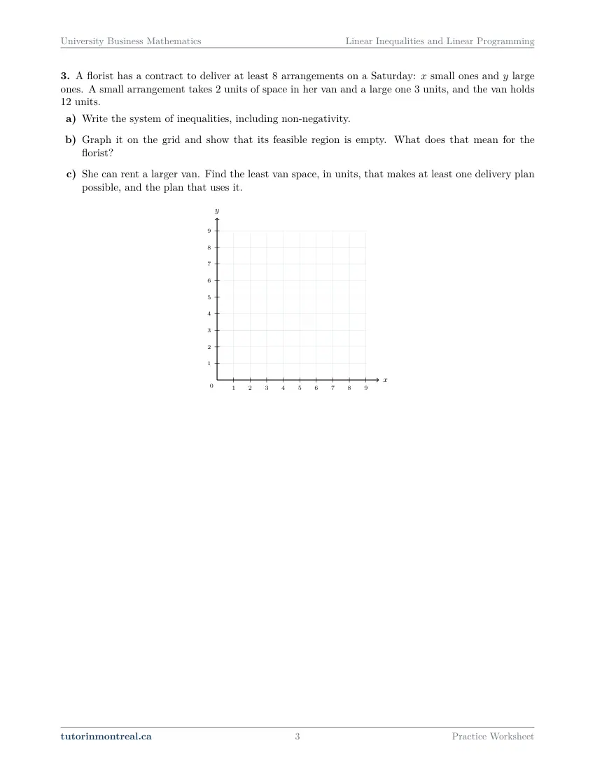
Q3 mixes directions. A contract for at least a certain number of arrangements gives a ≥ constraint; a van with limited space gives a ≤ one. When two constraints push in opposite directions, the region they share can shrink to nothing. Q3(b) asks you to show that happens here and to say what it means in plain words for the florist: a feasible region is a list of possible plans, and an empty one is a statement about the business, not a mistake in the algebra. Q3(c) turns the question around — the van capacity becomes the unknown. Ask which plan meeting the contract uses the least space, and let that plan set the capacity.
Corner points, bounded and unbounded
A corner point is a point of the feasible region where two boundary lines meet. Finding one is solving a system of two equations: pick the two boundary lines, replace each inequality by equality, and solve by substitution or elimination. Reading a corner off the grid is a check, never the method — corners rarely fall on grid points.
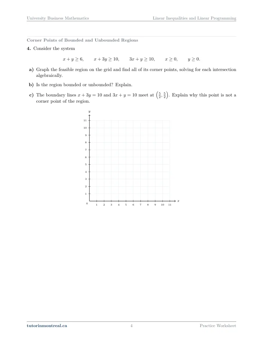
Not every intersection is a corner. Two boundary lines can meet at a point that some other constraint excludes. Before you list an intersection as a corner, test it in every constraint of the system. Q4(c) gives you exactly such a point and asks you to explain, from the constraints, why it is not a corner of the region.
Q4(a) has three ≥ constraints besides non-negativity, so the region lies on the far side of all three lines from the origin. Draw them, find which pairs of lines actually meet on the edge of the region, and solve each pair algebraically. Q4(b) asks whether the region is bounded. The test is geometric: a region is bounded when a circle could be drawn around all of it, and unbounded when it runs off in some direction without end. Decide from the constraints, not from how much of the region fits on the grid: ask whether some direction lets x or y grow as large as you like without breaking any inequality, and explain in a sentence either way.
Formulating a linear programming model
A linear programming model has three parts, and a complete answer writes all three before any graph is drawn.
From a story to a model
Write the parts in this order.
- 1Decision variables, with units
"Let x be the number of street decks assembled per week." A variable without its unit and time period is a common source of lost marks.
- 2The objective
Maximize profit or minimize cost, written as a linear function of the variables: amount per unit times the number of units, summed.
- 3Every constraint
One per resource (used ≤ available), one per order or requirement (at least means ≥, at most means ≤), and x ≥ 0, y ≥ 0.
Q5 has five constraints hiding in the story: two resource limits, a sales cap on one product, a standing order on the other, and non-negativity. A table with a row per resource and a column per product makes the coefficients easy to read off. The instruction "do not solve it" is part of the question — the formulation is the skill being checked. Q5(b) then tests one plan: check every constraint, and if the plan passes, evaluate the objective and subtract each resource used from what is available. That leftover amount is called slack, and it says which resources the plan leaves idle.
Q6 is a blending problem, and its difficulty is a percentage constraint. "At least a given percentage of the blend is protein" compares the protein in the feed with a fraction of the total tonnage x + y. Write protein from each ingredient on the left, the required fraction of x + y on the right, then collect everything on one side. Q6(a) wants the result with integer coefficients and zero on the right, so clear the decimals by multiplying through by a power of ten — a positive number, so the sign does not flip.
A percentage is a fraction of the total, not of one ingredient. Writing the protein requirement as a fraction of x alone, or of y alone, is the usual error in a blending problem. The total is x + y, and both variables appear on both sides before you simplify.
Solving a linear program graphically
The fundamental result of linear programming: if a linear objective has an optimal value on the feasible region, that value occurs at a corner point. So the graphical method is a finite search.
The corner-point method
Four steps once the model is written.
- 1Graph the feasible region
Every constraint, with its boundary and its side.
- 2Find every corner
Axis corners from intercepts; interior corners by solving the two boundary equations that meet there.
- 3Evaluate the objective at each corner
A table with a row per corner keeps the arithmetic honest.
- 4Read the answer in the story's words
How many of each product, and the profit or cost. If two adjacent corners tie, every point on the edge between them is optimal.
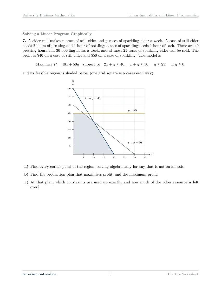
Q7 gives you the model and the shaded region, so the work starts at step 2. Its region has corners on both axes and others where two constraint lines cross, and those have to be solved for, not read off a grid whose squares are five cases wide. Q7(c) asks the follow-up a manager would ask: substitute the optimal plan into each constraint and see which ones hold with equality — those are the binding constraints, the resources the plan uses up — and how much of the remaining resource is left over.
Q8 is a minimization problem in which every requirement says "at least", so each constraint is a ≥ and the variables are what you buy rather than what you make. Q8(a) asks you to write the model, graph it and find the corners; Q8(b) is the corner-point method with cost in place of profit. Q8(c) asks why the cost has a minimum here but no maximum. The reason is about the direction the region opens: think about what happens to the cost as you buy more and more bags of either brand, and about which way the cost coefficients push.
Unbounded does not mean unsolvable. On an unbounded region, a minimization problem with positive cost coefficients always has a minimum at a corner, while a maximization problem may have no maximum at all. Checking a corner table alone cannot tell you which case you are in; you have to look at the direction the region runs off in.
The synthesis question
Q9 runs the whole chapter in one problem. Q9(a) is Q5's skill: variables with units, the profit objective, a constraint for peppers, a constraint for bottling minutes, the restaurant chain's order, and non-negativity. Watch the units — bottling time is given in minutes, and every term in that constraint must be in minutes too. Q9(b) is Q4's skill on a grid whose squares are five cases each way: draw the lines from their intercepts, then find the corners algebraically. Q9(c) is Q7's corner-point table, answered as a weekly plan and a profit.
Preview all 9 pages
Click any page to open the full PDF.
Getting the most out of it
Write the model before you draw anything
Variables with units, the objective, every constraint including non-negativity. A graph drawn from a half-written model has to be redrawn, and the formulation is marked on its own.
Solve for corners, check them on the graph
Every corner that is not on an axis comes from solving two boundary equations together. The graph tells you which two lines to pair; the algebra gives the coordinates. If the two disagree, one of them is wrong — find out which before evaluating anything.
Test every intersection in every constraint
A point where two lines cross is a corner only if it is feasible. Substituting it into the whole system takes a few seconds and removes the most common wrong entry in a corner table.
Answer in the business's words
The last line of a linear programming question is a decision: how many of each product, at what profit or cost, and which resources run out. A pair of coordinates on its own is not the answer the question asked for.
Want the solutions, or something more challenging?
The worksheet, the questions above and every explanation on this page stay free permanently. Three more PDFs exist for this topic — the worked answer key, a harder problem set, and the answer key to that. They come with the University Business Math Solutions Bundle, beside the unit notes and the unit test, which is what keeps the rest of the series free.
What else exists for Linear Inequalities and Linear Programming
Three PDFs · 12 pages · all three are in the bundle below.
- Answer key — 3 pages. All 9 questions worked step by step, including the restrictions and the justifications. Not a list of final answers.
- Challenge problems — 6 pages, 6 problems. A separate sheet at exam-plus difficulty covering the same 5 concepts. Harder than anything on the free sheet.
- Challenge answer key — 3 pages. Every challenge problem worked to the same standard, with the checks shown.
- PDF, letter size, print-ready.
The one thing that's for sale
Every University Business Math topic — the complete Solutions Bundle
One download, one payment, the whole program. For all 9 University Business Math units: the worksheet, the reference notes, the challenge set, the unit test and every answer key — including this one.
- Worked solutions, not answer lists — every step written out
- Covers the whole year's program at this level
- Less than the price of one hour of tutoring — for the entire year's solutions
Taking Secondary 1 Math as well? The Secondary 1 Math bundle covers all 15 of its units — 106 PDFs, 474 pages — on the same terms.
Taking Secondary 2 Math as well? The Secondary 2 Math bundle covers all 14 of its units — 98 PDFs, 449 pages — on the same terms.
Taking Secondary 3 Math as well? The Secondary 3 Math bundle covers all 11 of its units — 77 PDFs, 367 pages — on the same terms.
Taking Secondary 4 Math as well? The Secondary 4 Math bundle covers all 17 of its units — 122 PDFs, 466 pages — on the same terms.
Taking Secondary 5 Math as well? The Secondary 5 Math bundle covers all 21 of its units — 147 PDFs, 589 pages — on the same terms.
Taking CEGEP Calculus I as well? The CEGEP Calculus I bundle covers all 9 of its units — 72 PDFs, 371 pages — on the same terms.
Taking CEGEP Calculus II as well? The CEGEP Calculus II bundle covers all 8 of its units — 64 PDFs, 335 pages — on the same terms.
Taking CEGEP Linear Algebra as well? The CEGEP Linear Algebra bundle covers all 7 of its units — 56 PDFs, 298 pages — on the same terms.
Taking University Calculus III as well? The University Calculus III bundle covers all 9 of its units — 72 PDFs, 516 pages — on the same terms.
Taking University Linear Algebra as well? The University Linear Algebra bundle covers all 9 of its units — 72 PDFs, 496 pages — on the same terms.
Taking University Differential Equations as well? The University Differential Equations bundle covers all 9 of its units — 36 PDFs, 182 pages — on the same terms.
Taking University Introductory Statistics as well? The University Introductory Statistics bundle covers all 9 of its units — 36 PDFs, 186 pages — on the same terms.
Taking University Discrete Math as well? The University Discrete Math bundle covers all 9 of its units — 36 PDFs, 155 pages — on the same terms.
Taking AP Calculus AB as well? The AP Calculus AB bundle covers all 8 of its units — 64 PDFs, 527 pages — on the same terms.
Common questions
Is this worksheet really free?
Yes — the questions are on this page to read, and the PDF downloads directly, no email and no account. The one paid item is optional: the complete University Business Mathematics Solutions Bundle, which covers every set at this level.
Which university courses is this for?
The course codes listed on this page are taken from the public course calendars of universities that teach mathematics to management and commerce students. Each course orders and weights the chapters its own way, and some reach a chapter later or not at all — so check the outline for your own section to see where this set falls in your term.
What do I need to know before starting this set?
Secondary 5 mathematics: graphing a line from its intercepts, solving two linear equations together by substitution or elimination, and the rule that multiplying an inequality by a negative number reverses it. No calculus is used.
When is the boundary line solid, and when is it dashed?
Solid when the inequality is ≤ or ≥, because points on the line satisfy it; dashed when it is < or >. Business constraints are almost always ≤ or ≥, since using exactly all of a resource is allowed.
Why is the optimal value always at a corner?
The objective is linear, so moving along any edge of the feasible region makes it steadily increase, steadily decrease, or stay the same. It can therefore always be improved, or at least kept equal, by sliding to one end of the edge — and the ends of edges are the corners.
What if two corners give the same best value?
Then every point on the edge joining them gives that value too, and the problem has infinitely many optimal solutions. Report both corners and say that any point on the segment between them is optimal.
Does this set cover the simplex method?
No. Linear programming in this course is graphical and in two variables. The simplex method, tableaux, duality and sensitivity analysis are not part of this set or of the course it is written for.
Can teachers use this in class?
Yes. Print and photocopy it for your own classes freely — I just ask that the tutorinmontreal.ca footer stays on the page.
I'm stuck on one question. Can you help?
Yes — through one-on-one tutoring, in Montreal or online. Get in touch to arrange a session, or see the current rates.
← All 9 University Business Math worksheets · Secondary 1 Math series (15 sheets) → · Secondary 2 Math series (14 sheets) → · Secondary 3 Math series (11 sheets) → · Secondary 4 Math series (17 sheets) → · Secondary 5 Math series (21 sheets) → · CEGEP Calculus I series (9 sheets) → · CEGEP Calculus II series (8 sheets) → · CEGEP Linear Algebra series (7 sheets) → · University Calculus III series (9 sheets) → · University Linear Algebra series (9 sheets) → · University Differential Equations series (9 sheets) → · University Introductory Statistics series (9 sheets) → · University Discrete Math series (9 sheets) → · AP Calculus AB series (8 sheets) →