University Calculus III — Directional Derivatives and the Gradient Worksheet
The set where the partial derivatives stop being separate numbers and become one vector. Collecting them into the gradient and evaluating it at a point, then running that backwards to find where the gradient takes a given value; the rate of change of a function in any direction you choose, with the direction turned into a unit vector first and the units said out loud; the direction in which a function climbs fastest, how fast that is, and why no direction can do better; the gradient drawn on a grid at right angles to the level curve through its tail; and the tangent plane and normal line to a surface written as a level surface, with the gradient as its normal. A closing hillside question ties all of it to one map. Have a look on this page, then print the free PDF when you want to write on it.
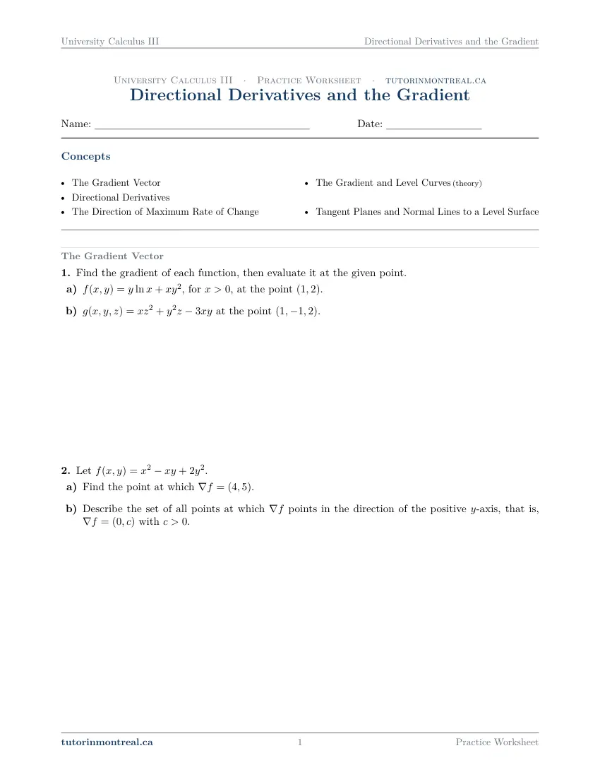
Practice worksheet — free PDF
No email, no account, no watermark. Teachers: photocopy it for your classes freely. Worked solutions and 7 harder problems come with the University Calculus III bundle.
All 10 questions
Each question targets one named concept from the sheet. Read them here, or print the PDF — it has working space under each one.
-
Q1The Gradient Vector
Find the gradient of each function, then evaluate it at the given point.
- , for , at the point .
- at the point .
-
Q2The Gradient Vector
Let .
- Find the point at which .
- Describe the set of all points at which points in the direction of the positive -axis, that is, with .
-
Q3Directional Derivatives
Find the directional derivative of at the point in the direction of . State whether is increasing or decreasing in that direction.
-
Q4Directional Derivatives
The concentration of a dye in a tank, in , is , with , , in centimetres.
- Find the rate of change of the concentration at the point in the direction from towards the point . Include units.
- A probe passes through heading towards at . At what rate, in per second, is the concentration it reads changing at that instant?
-
Q5The Direction of Maximum Rate of Change
Let , defined for . At the point , find the unit direction in which increases most rapidly and the maximum rate of increase. Then state the unit direction in which decreases most rapidly, and the value of the directional derivative of in that direction (a signed number).
-
Q6The Direction of Maximum Rate of Change
The temperature at the point of a heated plate is , in , with and in centimetres. An ant is at the point .
- In which unit direction should the ant set off to warm up as fast as possible, and what is that rate?
- The ant prefers to warm up at exactly . Find every unit direction that achieves this.
- Explain why no direction lets the ant warm up at .
-
Q7The Gradient and Level Curves
Let . On the grid below, the axes cross at the centre and each square is one unit, so the grid shows and .
- Write the equation of the level curve of that passes through the point , and sketch the part of it that fits on the grid.
- Compute and draw it on the grid with its tail at .
- Use the gradient to find the equation of the tangent line to the level curve at , and draw the line.
A blank Cartesian grid for this question is on the printable PDF.
-
Q8Tangent Planes and Normal Lines to a Level Surface
Find an equation of the tangent plane, and parametric equations of the normal line, to the surface at the point .
-
Q9Tangent Planes and Normal Lines to a Level Surface
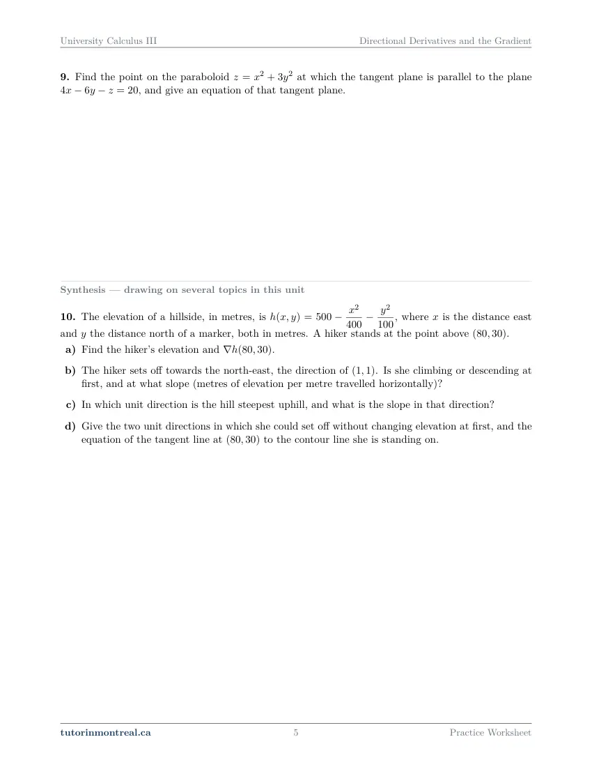
Find the point on the paraboloid at which the tangent plane is parallel to the plane , and give an equation of that tangent plane.
-
Q10Synthesis — drawing on several topics in this unit
The elevation of a hillside, in metres, is , where is the distance east and the distance north of a marker, both in metres. A hiker stands at the point above .
- Find the hiker's elevation and .
- The hiker sets off towards the north-east, the direction of . Is she climbing or descending at first, and at what slope (metres of elevation per metre travelled horizontally)?
- In which unit direction is the hill steepest uphill, and what is the slope in that direction?
- Give the two unit directions in which she could set off without changing elevation at first, and the equation of the tangent line at to the contour line she is standing on.
The 7 challenge problems for this topic are a separate, paid sheet and are not reproduced here.
What does this set assume? This set stands on CEGEP Calculus I, CEGEP Calculus II and CEGEP Linear Algebra, and on the previous set's partial derivatives, and re-teaches none of them. First-order partials of polynomial, root, logarithmic and rational functions, the norm of a vector, the dot product and the angle it measures, unit vectors, and the equations of a plane from a point and a normal and of a line from a point and a direction are all used without comment. Every function here is differentiable wherever it is used, and there is no epsilon-delta argument anywhere in the set. Scope is the gradient, directional derivatives, the direction and size of the maximum rate of change, the gradient as a normal to a level curve, and tangent planes and normal lines to a level surface. Critical points, the second derivative test and Lagrange multipliers belong to the optimisation set that follows, and potential functions — finding a function whose gradient is a given vector field — wait for the vector-field sets at the end of the course.
Which course is this for? In the public course calendars of Montreal universities, this material is part of the courses numbered MATH 222, MAST 218, ENGR 233, MAT1400, MAT1115, MTH1101 and MAT165. Each course orders and weights the topics its own way, so check your own outline for what your exam covers. Which sets match your course.
The rest of this unit
The worksheet is the practice, and it is free. Two more printable documents cover the same unit and come with the University Calculus III bundle: read the notes first, work this sheet, then sit the test closed-book. See what each one covers.
What the Directional Derivatives and the Gradient notes cover About the Directional Derivatives and the Gradient unit test
How to do every concept on this sheet
This is the part worksheet sites usually leave out. Below is the actual reasoning behind each group of questions — not a full solution set, the decisions that get you to one. Read it before you start, or after you get stuck.
The gradient vector: every partial derivative in one place
The gradient of f is the vector of its first-order partial derivatives, written in the order of the variables: two components for a function of x and y, three for a function of x, y and z. Q1 asks for the gradient of one function of each kind and then its value at a point, and there is nothing new in the calculus — each component is a partial derivative of the kind the previous set drilled. What is new is the bookkeeping.
∇f(x, y) = (fx, fy) ∇g(x, y, z) = (gx, gy, gz)Formula first, point second. Write the gradient as a vector of formulas, then substitute the point into every component. In part (a), the term y ln x is a product when you differentiate in x and a constant times ln x when you differentiate in y, so the two components need different rules. Note the stated domain, x > 0: the logarithm is what limits it. In part (b), keep track of which variable each term actually contains — a term with no z in it contributes nothing to the third component.
The answer is a vector, not a list of partials. Report the gradient at the point as one vector with its components in order. A function of three variables has a gradient in space, so an answer to part (b) with two components has lost one.
Q2 runs the gradient backwards. Part (a) gives the value of the gradient and asks where it is taken: setting each component equal to its target gives two linear equations in x and y, a small system of the kind Linear Algebra solves. Substitute your point back into the gradient to confirm it.
Part (b) asks for every point where the gradient points along the positive y-axis, which the question translates for you into a vector (0, c) with c > 0. That is two conditions, not one: an equation for the first component and an inequality for the second. Solve the equation, substitute what it gives into the second component, and then decide where the inequality holds. A description that uses only the first condition answers a different question. Say also what happens at any point where the whole gradient is zero, since the zero vector has no direction at all.
Directional derivatives: a rate of change in any direction
The partial derivatives are the rates of change along the two axes. The directional derivative is the rate of change along any direction, and for a differentiable function it comes from the gradient by one dot product — provided the direction is a unit vector.
Duf(P) = ∇f(P) · u, u a unit vectorComputing a directional derivative
Four steps, and the second is the one that gets skipped.
- 1Gradient at the point
Find ∇f as formulas, then evaluate at P.
- 2Make the direction a unit vector
Divide the given vector by its norm. A direction given as a vector of length other than 1 scales the answer by that length if you skip this.
- 3Dot product
Multiply matching components and add.
- 4Read the sign
Positive means the function increases in that direction, negative means it decreases.
Q3 is those four steps with a direction vector whose length is a whole number, so the unit vector has simple fractions. It then asks whether f is increasing or decreasing in that direction, and step 4 answers it: the sign of the directional derivative is the whole verdict. A useful check on the size of your answer comes from the next sheet — no directional derivative can be larger in absolute value than the norm of the gradient.
Q4 puts the same computation in space, with a dye concentration in a tank and the direction given as "from P towards Q" rather than as a vector.
A direction from P to Q is Q − P. The position vector of Q is not the direction of travel from P. Subtract, then normalise the difference. And part (a) asks for units: a directional derivative is a rate per unit of distance, so here it is milligrams per litre per centimetre.
From per centimetre to per second. Part (b) sends a probe through P at a given speed. The directional derivative tells you how much the reading changes for each centimetre travelled; the speed tells you how many centimetres pass each second. Multiplying the two converts a rate per unit distance into a rate per unit time — the one-variable chain rule in disguise. Check that the units come out as the question asks.
The direction of maximum rate of change
Writing the dot product with the angle θ between u and the gradient turns the directional derivative into a statement about geometry. Everything in this sheet follows from it.
Duf = ‖∇f‖ cos θ → largest when θ = 0, smallest when θ = π, zero when θ = π/2Q5 asks for four things at one point: the unit direction of fastest increase and the rate there, then the unit direction of fastest decrease and the directional derivative in it. The first pair is the gradient normalised, and its norm. The second pair is the opposite direction, and the question insists on a signed number: the directional derivative in the direction of fastest decrease is negative, because the function is falling there, even though the size of the fall is the same norm.
Simplify the root before you differentiate further. In Q5 both partials of the square root share the same denominator, and at the given point the expression under the root is a perfect square. Evaluate that once and reuse it in both components.
Q6 gives the temperature of a plate and an ant that wants to warm up. Part (a) is Q5's first half in a context: the ant should head along the gradient, and the rate is its norm, in degrees per centimetre. Part (b) turns the question round — a fixed rate is required, and you must find every unit direction that delivers it.
Two equations for an unknown unit vector. Write u = (p, q). The required rate gives one equation, ∇T · u equal to the target; being a unit vector gives the other, p² + q² = 1. Solve them together. A circle and a line usually meet twice, so expect more than one direction, and check each against both equations. The formula with cos θ gives the same answer from the angle, which is a good way to see why the directions come in a pair placed symmetrically about the gradient.
Part (c) is a proof, not a search. To show that no direction achieves a given rate, do not try directions until you give up. Use cos θ ≤ 1: every directional derivative at the point is at most the norm of the gradient, and compare the requested rate with that ceiling.
The gradient and level curves
The directions in which f does not change at all are the ones at right angles to the gradient, and those are the directions along the level curve. So at every point where it is not zero, the gradient is perpendicular to the level curve through that point. Q7 makes you draw this on a grid.
Q7 on the grid
A curve, an arrow, and a line that meets the arrow at a right angle.
- 1Which level?
Evaluate f at the given point. The level curve through it is f(x, y) equal to that number. Solve for y to sketch it, and plot enough points to show its shape inside the grid.
- 2Draw the gradient from the point
Evaluate ∇f at the point and draw it as an arrow with its tail there — move across by the first component and up by the second.
- 3Tangent line from a normal
The gradient is a normal vector to the tangent line, so the line is ∇f(a, b) · (x − a, y − b) = 0. Expand it and draw it.
- 4Look at the picture
The line should touch the curve at the point, and the arrow should meet the line at a right angle. If it does not, one of the three pieces is wrong.
The question asks for the gradient route. You can reach the same tangent line by solving for y and differentiating in one variable, and that makes a good check. It is not a substitute: part (c) says to use the gradient, and that is what is being marked.
Tangent planes and normal lines to a level surface
In three variables the same fact holds one dimension up: the gradient of F at a point is normal to the level surface of F through that point. The previous set wrote tangent planes only for graphs z = f(x, y); this one writes them for any surface given as an equation in x, y and z.
surface F(x, y, z) = k → normal n = ∇F(a, b, c) → plane n · (x − a, y − b, z − c) = 0, line (a, b, c) + t nQ8 is that chain applied once. Name the function F whose level surface the equation is, check that the given point is on it, compute ∇F there, and use it twice: as the normal of the plane and as the direction of the normal line.
Scale the normal before you use it. If every component of the gradient shares a factor, divide it out. Any non-zero multiple of a normal is a normal, and a smaller one gives a cleaner plane and a cleaner line. Write the normal line with its parameter and the range of the parameter.
Q9 is the same idea run in reverse, on a paraboloid given as z equal to a function of x and y. Move everything to one side so the paraboloid becomes a level surface of a function of three variables, and its gradient gives the normal at a general point, in terms of x and y.
parallel planes ⇔ parallel normals ⇔ ∇F = λ (normal of the given plane)Let the constant component fix the scalar. One component of the normal to the paraboloid does not depend on the point at all. Matching it with the corresponding component of the given plane's normal settles λ at once, and then the other two components give x and y. Find z from the surface's equation, not from the given plane — the point has to be on the paraboloid. Finally, compare your tangent plane with the given one: parallel planes share a normal, so they should differ only in the constant.
The synthesis question
Q10 puts the whole set on one hillside, with the elevation a function of distance east and distance north. Part (a) is Q1: the elevation at the hiker's position and the gradient there. Part (b) is Q3 — normalise the north-east direction, take the dot product, and let the sign say whether she climbs or descends; the slope is metres of elevation per metre travelled horizontally. Part (c) is Q5: the steepest uphill direction is the gradient normalised, and the slope in it is the gradient's norm. Part (d) joins the last two sheets: the directions in which the elevation does not change at first are the two unit vectors perpendicular to the gradient, and the contour line she stands on is the level curve through her position, so its tangent line has the gradient as its normal, exactly as in Q7.
Compare (b) with (c) before you move on. The slope in any direction lies between minus and plus the norm of the gradient. Seeing where your answer to (b) sits in that range, and comparing it with the angle between north-east and the gradient, is a check that costs one line.
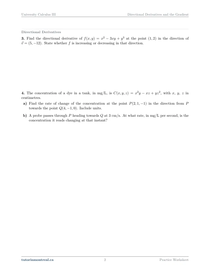
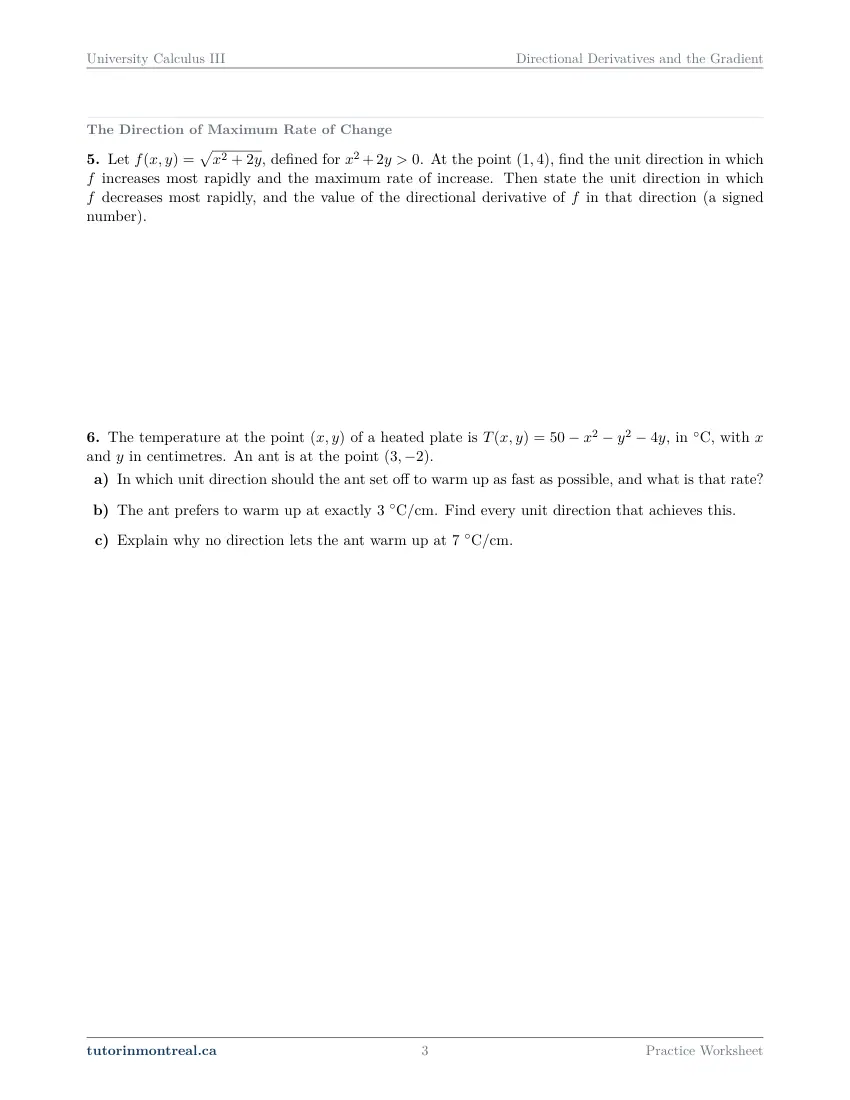
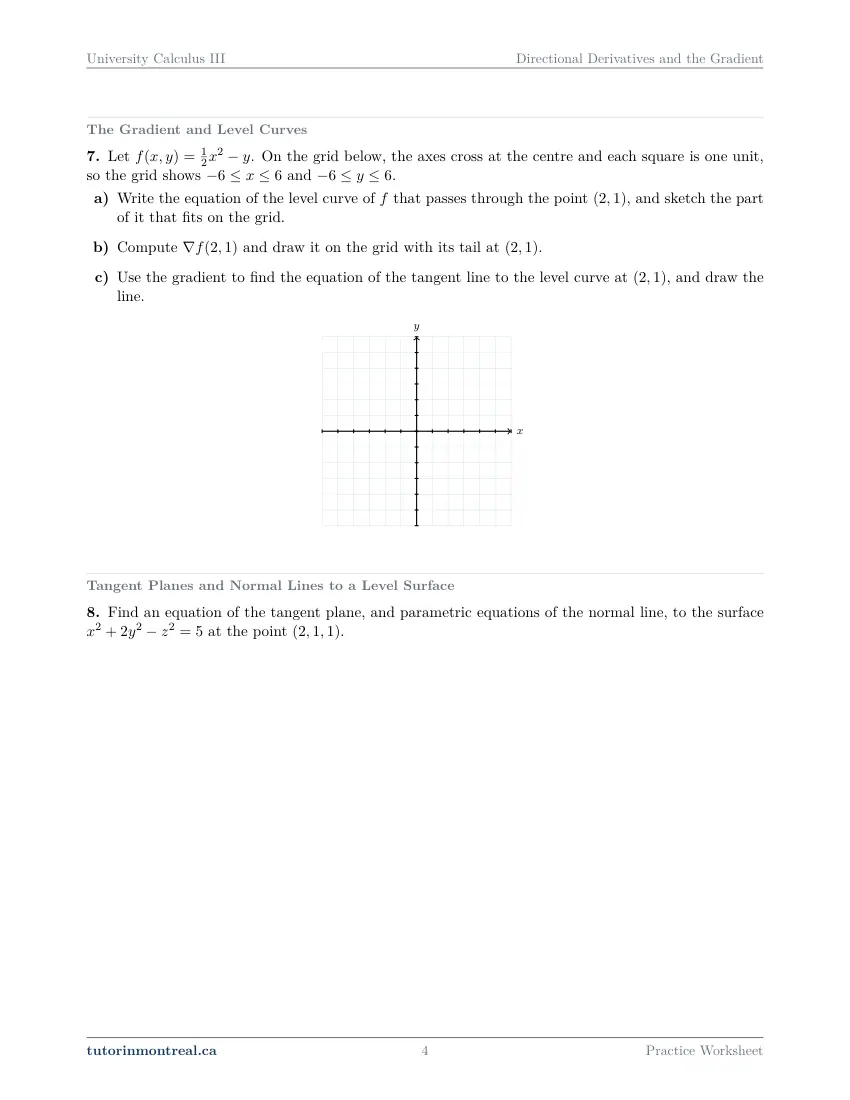
Preview all 6 pages
Click any page to open the full PDF.
Getting the most out of it
Normalise the direction before anything else
The formula Duf = ∇f · u is only true for a unit vector. Make it a habit to divide the given direction by its norm the moment you read it, and to write u with a small hat or the word "unit" beside it. Most lost marks in this topic are a missing division.
Check every rate against the norm of the gradient
Once you have ∇f at a point, you know the range every directional derivative there must lie in: from minus its norm to plus its norm. A directional derivative outside that range is wrong, and one exactly at an end of it means your direction is along the gradient or against it. It is a free check, so use it.
Draw the gradient on the level curve
Even when the question does not ask for a sketch, a rough picture of the level curve through the point with the gradient drawn from it shows at a glance which directions climb, which fall and which stay level. It also catches a gradient with a sign error, which will point downhill instead of up.
Write a surface as a level surface before looking for a normal
Whatever form the surface is given in, move everything to one side and name the function F. Then the normal is ∇F, with no special cases to remember, and the same recipe gives the tangent plane and the normal line.
Keep the units on every rate
A directional derivative is a rate per unit of distance. Writing the units forces you to notice when a question wants a rate per unit of time instead, as a moving probe or a walking hiker does, and to multiply by the speed.
Want the solutions, or something more challenging?
The worksheet, the questions above and every explanation on this page stay free permanently. Three more PDFs exist for this topic — the worked answer key, a harder problem set, and the answer key to that. They come with the University Calculus III Solutions Bundle, beside the unit notes and the unit test, which is what keeps the rest of the series free.
What else exists for Directional Derivatives and the Gradient
Three PDFs · 14 pages · all three are in the bundle below.
- Answer key — 3 pages. All 10 questions worked step by step, including the restrictions and the justifications. Not a list of final answers.
- Challenge problems — 7 pages, 7 problems. A separate sheet at exam-plus difficulty covering the same 5 concepts. Harder than anything on the free sheet.
- Challenge answer key — 4 pages. Every challenge problem worked to the same standard, with the checks shown.
- PDF, letter size, print-ready.
The one thing that's for sale
Every University Calculus III topic — the complete Solutions Bundle
One download, one payment, the whole program. For all 9 University Calculus III units: the worksheet, the reference notes, the challenge set, the unit test and every answer key — including this one.
- Worked solutions, not answer lists — every step written out
- Covers the whole year's program at this level
- Less than the price of one hour of tutoring — for the entire year's solutions
Taking Secondary 1 Math as well? The Secondary 1 Math bundle covers all 15 of its units — 106 PDFs, 474 pages — on the same terms.
Taking Secondary 2 Math as well? The Secondary 2 Math bundle covers all 14 of its units — 98 PDFs, 449 pages — on the same terms.
Taking Secondary 3 Math as well? The Secondary 3 Math bundle covers all 11 of its units — 77 PDFs, 367 pages — on the same terms.
Taking Secondary 4 Math as well? The Secondary 4 Math bundle covers all 17 of its units — 122 PDFs, 466 pages — on the same terms.
Taking Secondary 5 Math as well? The Secondary 5 Math bundle covers all 21 of its units — 147 PDFs, 589 pages — on the same terms.
Taking CEGEP Calculus I as well? The CEGEP Calculus I bundle covers all 9 of its units — 72 PDFs, 371 pages — on the same terms.
Taking CEGEP Calculus II as well? The CEGEP Calculus II bundle covers all 8 of its units — 64 PDFs, 335 pages — on the same terms.
Taking CEGEP Linear Algebra as well? The CEGEP Linear Algebra bundle covers all 7 of its units — 56 PDFs, 298 pages — on the same terms.
Taking University Linear Algebra as well? The University Linear Algebra bundle covers all 9 of its units — 72 PDFs, 496 pages — on the same terms.
Taking University Differential Equations as well? The University Differential Equations bundle covers all 9 of its units — 36 PDFs, 182 pages — on the same terms.
Taking University Business Math as well? The University Business Math bundle covers all 9 of its units — 36 PDFs, 190 pages — on the same terms.
Taking University Introductory Statistics as well? The University Introductory Statistics bundle covers all 9 of its units — 36 PDFs, 186 pages — on the same terms.
Taking University Discrete Math as well? The University Discrete Math bundle covers all 9 of its units — 36 PDFs, 155 pages — on the same terms.
Taking AP Calculus AB as well? The AP Calculus AB bundle covers all 8 of its units — 64 PDFs, 527 pages — on the same terms.
Common questions
Is this worksheet really free?
Yes — the questions are on this page to read, and the PDF downloads directly, no email and no account. The one paid item is optional: the complete University Calculus III Solutions Bundle, which covers every set at this level.
Which university courses is this for?
The course codes listed on this page are taken from the public course calendars of universities that teach multivariable calculus after CEGEP. Each course orders and weights the topics its own way — some treat the gradient together with partial derivatives, some give tangent planes to level surfaces a week of their own — so check the outline for your own section to see where this set falls in your term.
What do I need to know before starting this set?
CEGEP Calculus I and II, CEGEP Linear Algebra, and the previous set on partial derivatives. You should be comfortable computing first-order partials, finding the norm of a vector and a dot product, turning a vector into a unit vector, and writing a plane from a point and a normal and a line from a point and a direction.
Why does the direction have to be a unit vector?
Because a directional derivative is a rate per unit of distance travelled. The dot product of the gradient with a longer vector is multiplied by that vector's length, so it measures the change over a longer step rather than the rate. Dividing by the norm removes the length and keeps only the direction.
What is the difference between the gradient and a directional derivative?
The gradient is a vector, one at each point, that holds all the first-order partial derivatives. A directional derivative is a single number, the rate of change in one chosen direction, and you get it from the gradient by a dot product with a unit vector. The gradient's own direction is the one in which that number is largest, and its norm is that largest value.
Why is the gradient perpendicular to a level curve?
Along a level curve the function does not change, so the directional derivative in the direction of the curve is zero. A zero dot product means the gradient is at right angles to that direction. The same argument in three variables makes the gradient normal to a level surface, which is why it gives the tangent plane.
How is this tangent plane different from the one in the partial derivatives set?
The earlier set wrote tangent planes only to graphs z = f(x, y). Here any surface given by an equation in x, y and z can be treated as a level surface of a function F, and its gradient is the normal. A graph is one special case of a level surface, so the two methods agree whenever both apply.
Where are critical points and Lagrange multipliers?
In the next set, on optimisation. They are built on the gradient — a critical point is where it is zero, and Lagrange multipliers compare two gradients — which is why this set comes first.
Can teachers use this in class?
Yes. Print and photocopy it for your own classes freely — I just ask that the tutorinmontreal.ca footer stays on the page.
I'm stuck on one question. Can you help?
Yes — through one-on-one tutoring, in Montreal or online. Get in touch to arrange a session, or see the current rates.
← All 9 University Calculus III worksheets · Secondary 1 Math series (15 sheets) → · Secondary 2 Math series (14 sheets) → · Secondary 3 Math series (11 sheets) → · Secondary 4 Math series (17 sheets) → · Secondary 5 Math series (21 sheets) → · CEGEP Calculus I series (9 sheets) → · CEGEP Calculus II series (8 sheets) → · CEGEP Linear Algebra series (7 sheets) → · University Linear Algebra series (9 sheets) → · University Differential Equations series (9 sheets) → · University Business Math series (9 sheets) → · University Introductory Statistics series (9 sheets) → · University Discrete Math series (9 sheets) → · AP Calculus AB series (8 sheets) →