University Calculus III — Vector Fields and Line Integrals Worksheet

10 of the 13 questions

Each question targets one named concept from the sheet. Read them here, or print the PDF — it has working space under each one. 10 of the 13 questions are printed below. The other 3 are built on a diagram or a table of values that does not translate to the page, so they are in the free PDF — marked below where they would have come.

1. Q1Vector Fields

   Let $\overrightarrow{F}(x,y)=(\frac{1}{2}y,-\frac{1}{2}x)$.

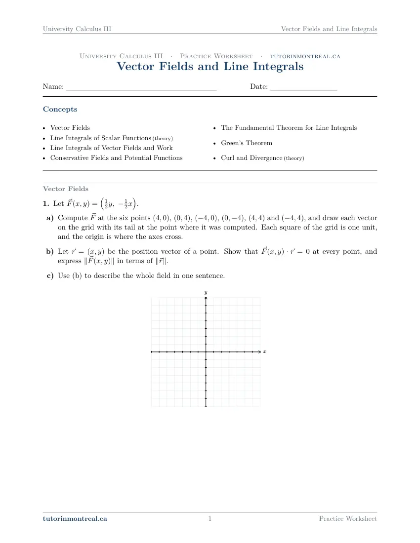
   1. Compute $\overrightarrow{F}$ at the six points $(4,0)$, $(0,4)$, $(-4,0)$, $(0,-4)$, $(4,4)$ and $(-4,4)$, and draw each vector on the grid with its tail at the point where it was computed. Each square of the grid is one unit, and the origin is where the axes cross.
   2. Let $\overrightarrow{r}=(x,y)$ be the position vector of a point. Show that $\overrightarrow{F}(x,y)·\overrightarrow{r}=0$ at every point, and express $\Vert \overrightarrow{F}(x,y)\Vert$ in terms of $\Vert \overrightarrow{r}\Vert$.
   3. Use (b) to describe the whole field in one sentence.

   A blank Cartesian grid for this question is on the printable PDF.

2. Q2Vector Fields

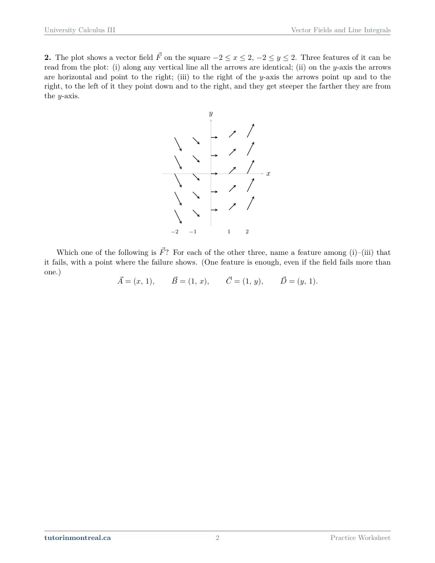
   This question is built around a diagram or a table of values. Open it in the PDF.

3. Q3Line Integrals of Scalar Functions

   A thin wire lies along the curve $\overrightarrow{r}(t)=(\frac{1}{3}{t}^3,t^2,2t)$, $0\le t\le 2$, with lengths in centimetres. Its linear density at the point $(x,y,z)$ is $\delta (x,y,z)=z$ grams per centimetre.

   1. Show that $\Vert \overrightarrow{r}{}^{\prime }(t)\Vert =t^2+2$.
   2. Find the mass of the wire, ${\displaystyle {\int }_C\delta ds}$.
   3. Find the length of the wire and hence its average density.
4. Q4Line Integrals of Vector Fields and Work

   A force field $\overrightarrow{F}(x,y)=(xy,x-y)$, in newtons, acts on a particle that moves along the parabola $y=x^2$ from $(0,0)$ to $(2,4)$, with distances in metres. Find the work done by $\overrightarrow{F}$, $W={\displaystyle {\int }_C\overrightarrow{F}·d\overrightarrow{r}}$.

5. Q5Line Integrals of Vector Fields and Work

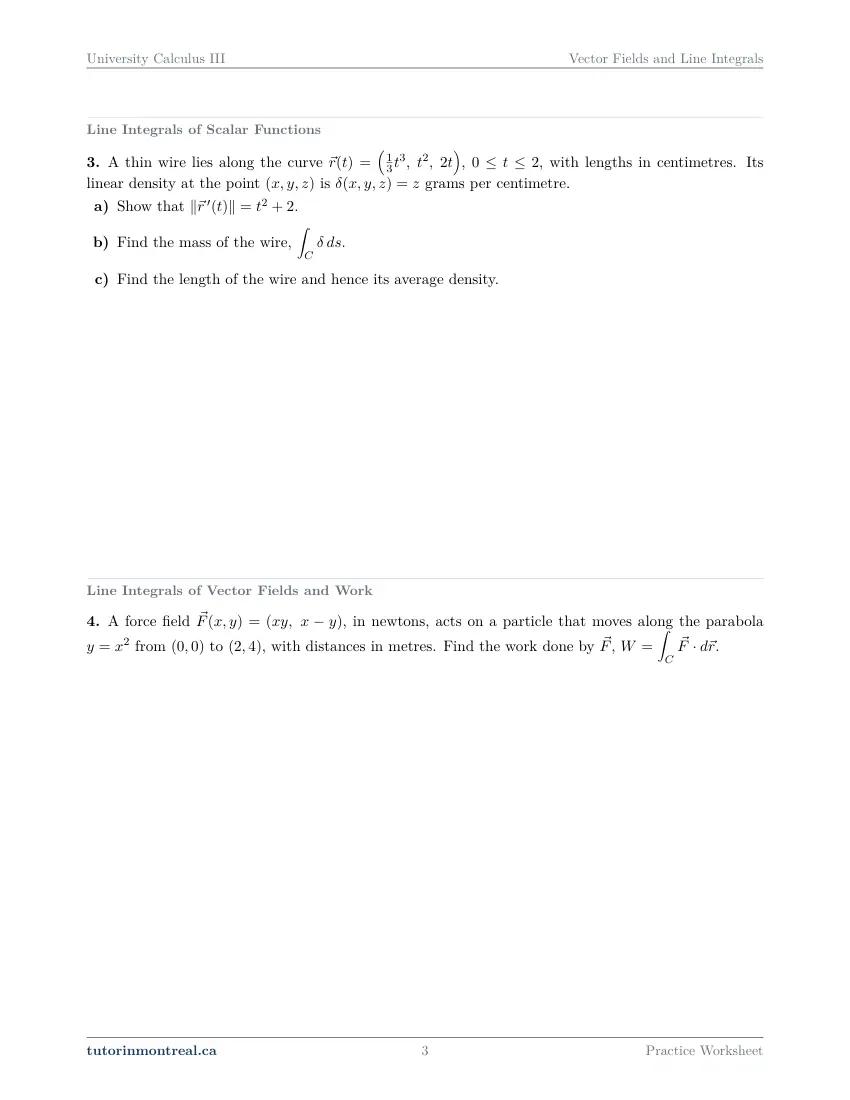
   This question is built around a diagram or a table of values. Open it in the PDF.

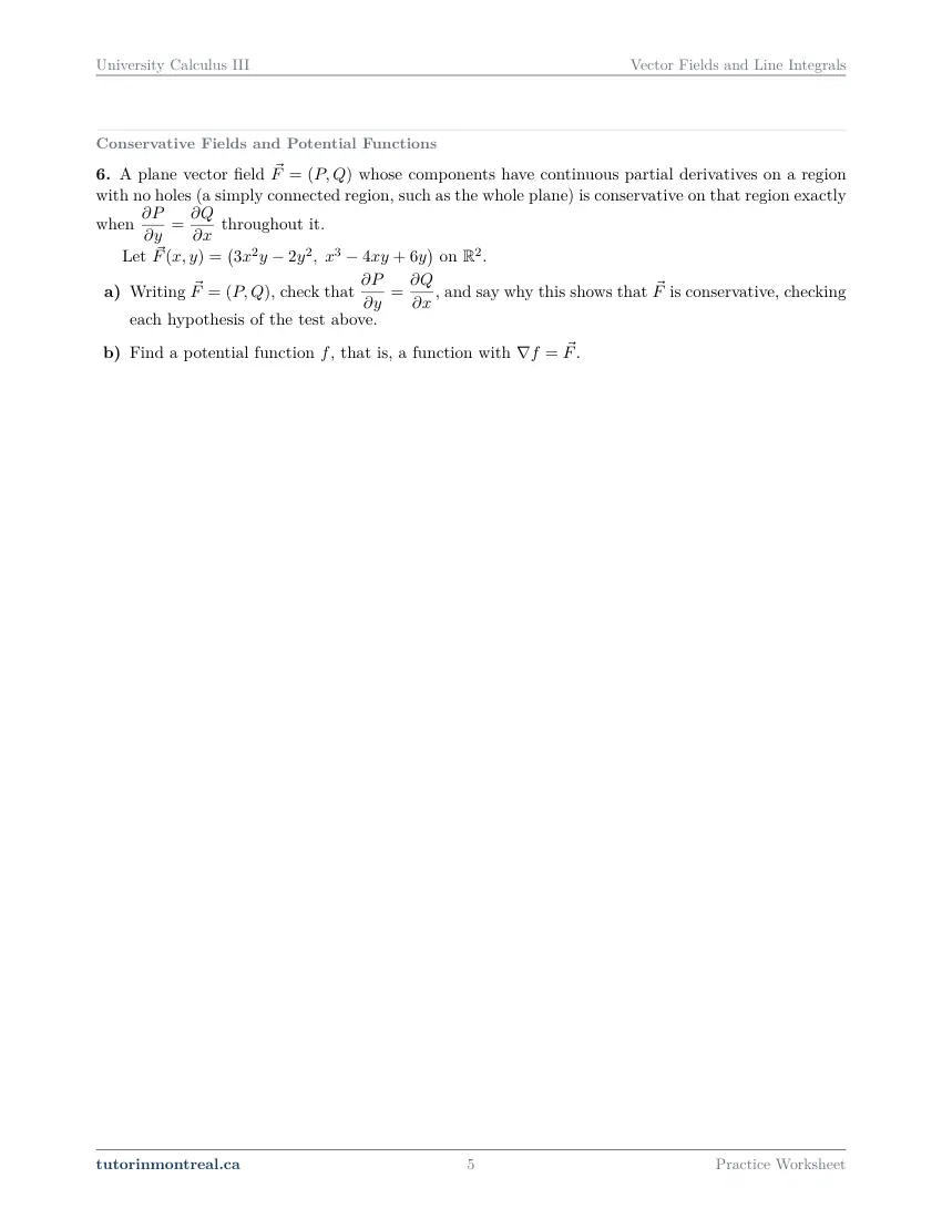
6. Q6Conservative Fields and Potential Functions

   A plane vector field $\overrightarrow{F}=(P,Q)$ whose components have continuous partial derivatives on a region with no holes (a simply connected region, such as the whole plane) is conservative on that region exactly when ${\displaystyle \frac{\partial P}{\partial y}}={\displaystyle \frac{\partial Q}{\partial x}}$ throughout it.

   Let $\overrightarrow{F}(x,y)=(3x^{2}y-2y^2,x^3-4xy+6y)$ on ${ℝ}^2$.

   1. Writing $\overrightarrow{F}=(P,Q)$, check that ${\displaystyle \frac{\partial P}{\partial y}}={\displaystyle \frac{\partial Q}{\partial x}}$, and say why this shows that $\overrightarrow{F}$ is conservative, checking each hypothesis of the test above.
   2. Find a potential function $f$, that is, a function with $\nabla f=\overrightarrow{F}$.
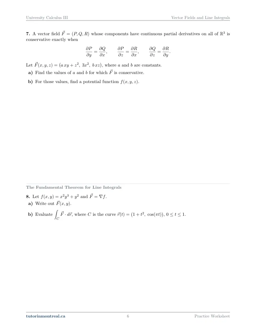
7. Q7Conservative Fields and Potential Functions

   A vector field $\overrightarrow{F}=(P,Q,R)$ whose components have continuous partial derivatives on all of ${ℝ}^3$ is conservative exactly when $$\frac{\partial P}{\partial y}=\frac{\partial Q}{\partial x},\frac{\partial P}{\partial z}=\frac{\partial R}{\partial x},\frac{\partial Q}{\partial z}=\frac{\partial R}{\partial y}.$$ Let $\overrightarrow{F}(x,y,z)=(axy+z^2,3x^2,bxz)$, where $a$ and $b$ are constants.

   1. Find the values of $a$ and $b$ for which $\overrightarrow{F}$ is conservative.
   2. For those values, find a potential function $f(x,y,z)$.
8. Q8The Fundamental Theorem for Line Integrals

   Let $f(x,y)=x^2{y}^3+y^2$ and $\overrightarrow{F}=\nabla f$.

   1. Write out $\overrightarrow{F}(x,y)$.
   2. Evaluate ${\displaystyle {\int }_C\overrightarrow{F}·d\overrightarrow{r}}$, where $C$ is the curve $\overrightarrow{r}(t)=(1+t^2,\cos (\pi t))$, $0\le t\le 1$.
9. Q9The Fundamental Theorem for Line Integrals

   The force field $\overrightarrow{F}(x,y,z)=(yz,xz,xy+2z)$, in newtons, has the potential function $f(x,y,z)=xyz+z^2$; distances are in metres. Let $A=(1,2,0)$, $B=(2,1,3)$ and $D=(0,5,1)$.

   1. Verify that $\nabla f=\overrightarrow{F}$.
   2. Find the work done by $\overrightarrow{F}$ on a particle that moves from $A$ to $B$ along any smooth curve.
   3. The particle then continues from $B$ to $D$. Find the work done on this second leg, and the total work from $A$ to $D$.
   4. How much work does $\overrightarrow{F}$ do on a particle that leaves $A$ and returns to $A$?
10. Q10Green's Theorem

    Let $C$ be the boundary of the triangle with vertices $(0,0)$, $(3,0)$ and $(0,3)$, traversed counterclockwise. Use Green's theorem to evaluate $${\oint }_C{y}^{2}dx+3xydy.$$

11. Q11Green's Theorem

    This question is built around a diagram or a table of values. Open it in the PDF.

12. Q12Curl and Divergence

    Let $\overrightarrow{F}(x,y,z)=(x^{2}y,y{z}^2,xz-y)$.

    1. Compute the divergence $\nabla ·\overrightarrow{F}$ and the curl $\nabla \times \overrightarrow{F}$.
    2. Evaluate both at the point $(1,-1,2)$.
    3. Is $\overrightarrow{F}$ conservative? Give the reason.
13. Q13Synthesis — drawing on several topics in this unit

    A force field $\overrightarrow{F}(x,y)=(2xy,x^2+3x)$, in newtons, acts in the plane; distances are in metres.

    1. Show that $\overrightarrow{F}$ is not conservative.
    2. Use Green's theorem to find the work done by $\overrightarrow{F}$ on a particle that goes once counterclockwise round the circle $x^2+y^2=4$.
    3. Find the work done by $\overrightarrow{F}$ along the diameter from $(-2,0)$ to $(2,0)$.
    4. Deduce, using Green's theorem on the upper half-disk, the work done along the upper semicircle from $(2,0)$ counterclockwise to $(-2,0)$.

The 9 challenge problems for this topic are a separate, paid sheet and are not reproduced here.

The rest of this unit

The worksheet is the practice, and it is free. Two more printable documents cover the same unit and come with the University Calculus III bundle: read the notes first, work this sheet, then sit the test closed-book. See what each one covers.

What the Vector Fields and Line Integrals notes cover  About the Vector Fields and Line Integrals unit test

How to do every concept on this sheet

This is the part worksheet sites usually leave out. Below is the actual reasoning behind each group of questions — not a full solution set, the decisions that get you to one. Read it before you start, or after you get stuck.

A vector field is a vector attached to every point

Q1 gives a plane field by its formula and asks you to compute it at six points and draw each vector with its tail at the point where it was computed. That last instruction is the whole convention: the arrow at (4, 4) starts at (4, 4), not at the origin. The grid is one unit per square, so each arrow is drawn by moving its two components from its own point.

Q2 runs the other way: a plot, shown in the PDF, and four candidate formulas. The question lists three features you can read from the plot, and asks you to pick the one formula that matches and, for each of the other three, to name one feature it fails and a point where the failure shows.

Line integrals of scalar functions

Q3 is a wire in space with a density that varies along it, and the mass is the integral of the density with respect to arc length. Everything is converted to the parameter t: the density is evaluated on the curve, and ds becomes the speed times dt.

Line integrals of vector fields and work

Work adds up the component of the force along the direction of travel, so the integrand is a dot product with r′(t), not a length. Q4 is the direct case: a force along a parabola from one point to another. Parametrize the parabola with x as the parameter, evaluate the field on the curve, dot it with the derivative, and integrate between the parameter values of the two endpoints.

Q5 is built on a figure, shown in the PDF: a curve in two pieces, a quarter circle followed by a straight segment. A line integral over a piecewise curve is the sum of the integrals over the pieces, each with a parametrization of its own.

Conservative fields and potential functions

A field is conservative when it is the gradient of some function f, its potential. Q6 states the test for a plane field and asks you to use it with its hypotheses: compare ∂P/∂y with ∂Q/∂x, and say why equality settles the matter here — the components have continuous partial derivatives, and the region is the whole plane, which has no holes.

Q7 is the same machinery in three dimensions, with two constants left open. There are three cross-partial conditions in space, and each one is an equation that must hold at every point: compare coefficients, and note which conditions hold whatever the constants are. Only once the constants are fixed is there a field to find a potential for in part (b).

The fundamental theorem for line integrals

When the field is a gradient, the line integral is the change in the potential between the endpoints — the path in between does not enter. Q8 hands you the potential and a curve whose parametrization would be unpleasant to integrate along. Part (a) is the gradient; for part (b), the only thing you need from the curve is where it starts and where it ends.

Q9 is the physical reading: a force field with a stated potential, three points in space, and work in joules. Part (a) verifies the potential; after that every part is a subtraction of two values of f. Part (c) asks for two legs and the total, which is a check in itself — the total must equal the difference between the last point and the first. Part (d) is the same subtraction with a special pair of endpoints.

Green's theorem

Green's theorem trades a line integral round a closed curve for a double integral over the region inside it. It needs a simple closed curve, traversed counterclockwise, and components with continuous partial derivatives on the region.

Q10 is the direct case: the boundary of a triangle, counterclockwise, with the integral written in P dx + Q dy form. Name P and Q, form ∂Q/∂x − ∂P/∂y, and describe the triangle by vertical or horizontal strips, as in the double-integrals set. The integrand that survives is usually simpler than either P or Q, which is the point of the theorem.

Q11 is built on a figure, shown in the PDF: a half-disk whose boundary is traversed clockwise. Two decisions carry it. First, why Green's theorem at all — look at which terms of P and Q a direct evaluation would have to antidifferentiate, and at what happens to each of them when you form ∂Q/∂x − ∂P/∂y. Second, the orientation: the theorem is stated for the counterclockwise boundary, and the curve here goes the other way.

Curl and divergence

Q12 asks for both of the derivatives a space field has. Divergence is a scalar: the sum of each component differentiated in its own variable. Curl is a vector, most reliably computed as the formal determinant of a 3 × 3 array with the unit vectors in the first row, the partial derivative operators in the second and the components in the third.

Part (c) asks whether the field is conservative, with the reason. The curl of a gradient field is the zero vector, because each of its components is a difference of mixed partial derivatives that are equal. So the curl you computed in part (a) is the test: decide whether it is the zero vector everywhere, and say which way that settles the question.

The synthesis question

Q13 follows one force field through four tools. Part (a) is Q6's test, used in the other direction: showing that ∂P/∂y and ∂Q/∂x are not equal is enough to rule out a potential, with no hypothesis about the region to check. Part (b) is Q10's method on a disk; look at what ∂Q/∂x − ∂P/∂y turns out to be, and the double integral may need nothing more than an area. Part (c) is Q4's method on a segment of the x-axis: parametrize it and notice what happens to the dy term there. Part (d) puts (b) and (c) together — the semicircle and the diameter close up into the boundary of a half-disk, so Green's theorem on that half-disk gives their sum, and subtracting the diameter's contribution leaves the semicircle's.

Preview all 10 pages

Click any page to open the full PDF.

Getting the most out of it

Decide the tool before you parametrize

Before any computation, ask three questions in order: is the field a gradient, is the curve closed, and is what is left simple to parametrize? A gradient means only endpoints; a closed curve means Green's theorem may be shorter; only when neither helps is a direct parametrization the right move.

Check every parametrization at both ends

Put the first and last parameter values into r(t) and compare them with the curve's stated start and end points. Half the sign errors in this block come from a parametrization that runs the right curve the wrong way.

Write ds and dr differently, on purpose

ds is the speed ‖r′(t)‖ dt, a positive length; dr is the vector r′(t) dt. Writing which one you are using at the top of each integral keeps a scalar integral from picking up an orientation, and a work integral from losing one.

Draw the orientation on the region for Green's theorem

Sketch the region, put an arrow on its boundary, and check that the region is on your left as you walk along it. If the curve in the question goes the other way, write the sign change down before you start the double integral, not after.

Verify a potential by taking its gradient

A potential function is checked in one line: differentiate it in each variable and compare with the components of the field. It costs less than any other check in this set and catches a forgotten h(y) every time.

Common questions