University Calculus III — Optimization in Several Variables Worksheet

All 11 questions

Each question targets one named concept from the sheet. Read them here, or print the PDF — it has working space under each one.

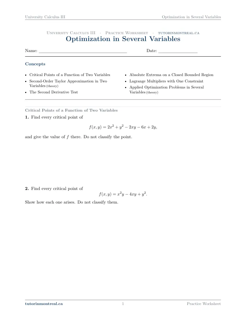
1. Q1Critical Points of a Function of Two Variables

   Find every critical point of $$f(x,y)=2x^2+y^2-2xy-6x+2y,$$ and give the value of $f$ there. Do not classify the point.

2. Q2Critical Points of a Function of Two Variables

   Find every critical point of $$f(x,y)=x^{2}y-4xy+y^2.$$ Show how each one arises. Do not classify them.

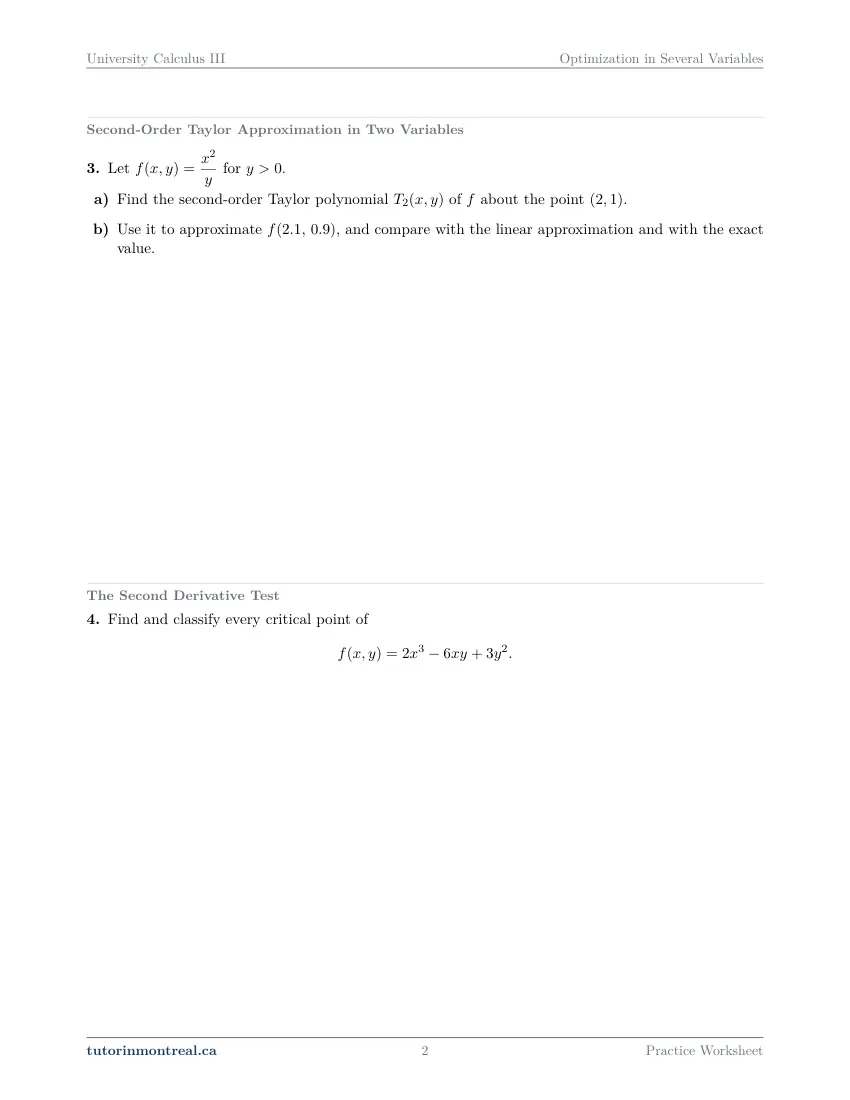
3. Q3Second-Order Taylor Approximation in Two Variables

   Let $f(x,y)={\displaystyle \frac{x^2}{y}}$ for $y>0$.

   1. Find the second-order Taylor polynomial $T_2(x,y)$ of $f$ about the point $(2,1)$.
   2. Use it to approximate $f(2.1,0.9)$, and compare with the linear approximation and with the exact value.
4. Q4The Second Derivative Test

   Find and classify every critical point of $$f(x,y)=2x^3-6xy+3y^2.$$

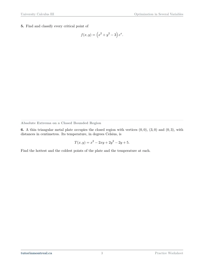
5. Q5The Second Derivative Test

   Find and classify every critical point of $$f(x,y)=(x^2+y^2-3)e^x.$$

6. Q6Absolute Extrema on a Closed Bounded Region

   A thin triangular metal plate occupies the closed region with vertices $(0,0)$, $(3,0)$ and $(0,3)$, with distances in centimetres. Its temperature, in degrees Celsius, is $$T(x,y)=x^2-2xy+2y^2-2y+5.$$ Find the hottest and the coldest points of the plate and the temperature at each.

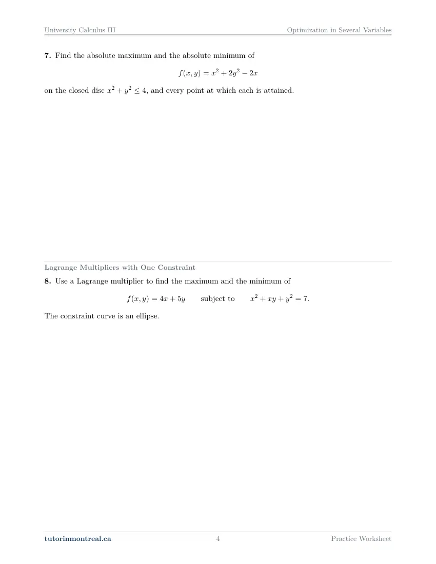
7. Q7Absolute Extrema on a Closed Bounded Region

   Find the absolute maximum and the absolute minimum of $$f(x,y)=x^2+2y^2-2x$$ on the closed disc $x^2+y^2\le 4$, and every point at which each is attained.

8. Q8Lagrange Multipliers with One Constraint

   Use a Lagrange multiplier to find the maximum and the minimum of $$f(x,y)=4x+5y\text{subject to}{x}^2+xy+y^2=7.$$ The constraint curve is an ellipse.

9. Q9Lagrange Multipliers with One Constraint

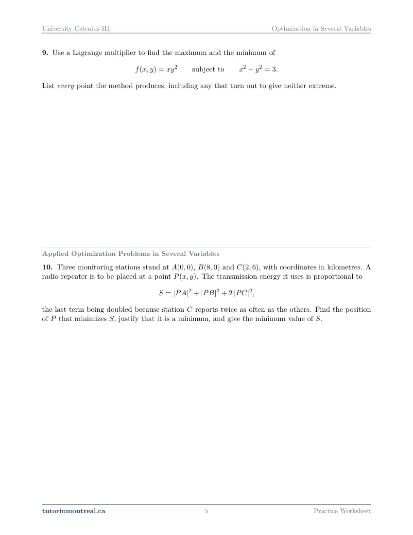
   Use a Lagrange multiplier to find the maximum and the minimum of $$f(x,y)=x{y}^2\text{subject to}{x}^2+y^2=3.$$ List every point the method produces, including any that turn out to give neither extreme.

10. Q10Applied Optimization Problems in Several Variables

    Three monitoring stations stand at $A(0,0)$, $B(8,0)$ and $C(2,6)$, with coordinates in kilometres. A radio repeater is to be placed at a point $P(x,y)$. The transmission energy it uses is proportional to $$S=|PA{|}^2+|PB{|}^2+2|PC{|}^2,$$ the last term being doubled because station $C$ reports twice as often as the others. Find the position of $P$ that minimizes $S$, justify that it is a minimum, and give the minimum value of $S$.

11. Q11Synthesis — drawing on several topics in this unit

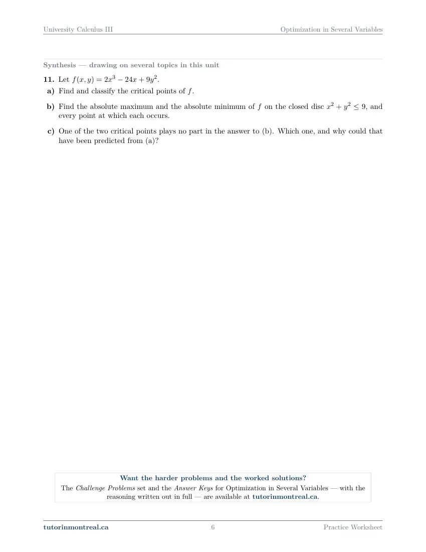
    Let $f(x,y)=2x^3-24x+9y^2$.

    1. Find and classify the critical points of $f$.
    2. Find the absolute maximum and the absolute minimum of $f$ on the closed disc $x^2+y^2\le 9$, and every point at which each occurs.
    3. One of the two critical points plays no part in the answer to (b). Which one, and why could that have been predicted from (a)?

The 8 challenge problems for this topic are a separate, paid sheet and are not reproduced here.

The rest of this unit

The worksheet is the practice, and it is free. Two more printable documents cover the same unit and come with the University Calculus III bundle: read the notes first, work this sheet, then sit the test closed-book. See what each one covers.

What the Optimization in Several Variables notes cover  About the Optimization in Several Variables unit test

How to do every concept on this sheet

This is the part worksheet sites usually leave out. Below is the actual reasoning behind each group of questions — not a full solution set, the decisions that get you to one. Read it before you start, or after you get stuck.

Critical points: where the gradient is zero

At a local maximum or minimum inside the domain, the surface has a horizontal tangent plane, so both first-order partial derivatives are zero there. For the polynomial functions of this sheet the partials exist everywhere, and finding the critical points means solving the system f_x = 0, f_y = 0 — every solution of it, not just the first one you see.

Q1 gives a quadratic polynomial, so both partials are linear and the system is two linear equations in x and y. Solve it by elimination, then substitute the point back into both partials to confirm each is zero. The question also asks for the value of f at the point and says not to classify it — that comes two sheets later.

Second-order Taylor approximation in two variables

The tangent plane is the best linear approximation to f near a point. Adding the three second-order terms gives the best quadratic one, the second-order Taylor polynomial. Write h and k for the displacements from the point (a, b), and evaluate every derivative at (a, b).

Part (b) asks for a comparison with the linear approximation and with the exact value, and the comparison is the point: keeping the linear part and the quadratic correction separate lets you see how much the second-order terms buy you, and computing the exact value tells you how close each approximation came.

The second derivative test

Near a critical point the first-order terms of T₂ vanish, so the shape of the graph there is decided by the quadratic part. The second derivative test reads its sign from one number.

Q4 is the whole routine on a cubic. The two first-order equations each give y in terms of x; setting the two expressions equal gives an equation in x alone, and its solutions give the critical points. Then compute the three second partials as formulas, write D as a formula in x and y, and evaluate it at each point in turn.

Q5 puts a polynomial in front of an exponential, so both partials come from the product rule and both carry the exponential as a factor.

Absolute extrema on a closed bounded region

A continuous function on a closed bounded region has an absolute maximum and an absolute minimum — the two-variable extreme value theorem — and each is attained either at a critical point inside the region or somewhere on its boundary. That turns the search into a finite list of candidates.

Q6 is a plate shaped like a triangle, so the boundary is three line segments, and each needs its own description: two of them are pieces of the axes, and the third is the slanted edge, written as y in terms of x over the interval the edge covers. Along each edge the temperature becomes a quadratic in one variable, whose vertex may or may not lie inside the edge's interval. The three corners are candidates too. Answer in the question's terms: where the hottest and coldest points are, and the temperature, in degrees Celsius, at each.

Q7 replaces the triangle with a disc. On its boundary circle, solve the circle's equation for y² and substitute: f becomes a function of x alone, on the interval of x-values the circle covers.

Lagrange multipliers with one constraint

To find the extremes of f along a curve g(x, y) = c, look for the points where the level curve of f touches the constraint curve instead of crossing it. There the two curves share a normal, so the two gradients are parallel.

In Q8 the objective is linear and the constraint is an ellipse. Before dividing one component equation by the other, show that λ cannot be zero; then the two equations give y as a multiple of x, and the constraint gives the candidates.

Q9 asks you to list every point the method produces, including any that give neither extreme. One of the component equations has a common factor on both sides.

Applied optimisation in several variables

In an applied problem the function is not given — you build it. Q10 places a repeater among three stations and asks for the position that minimises a weighted sum of squared distances, with the third station's term counted twice.

The synthesis question

Q11 uses one cubic-plus-quadratic function for two of the sheets. Part (a) is Q4: find the critical points and classify each with D. Part (b) is Q7 on a larger disc: check which critical points lie inside it, reduce the function on the boundary circle to one variable, keep only the critical numbers that fall inside the interval of x-values, test the interval's endpoints, and report every point at which each extreme occurs. A Lagrange multiplier on the circle is an alternative for the boundary, and it reaches the same candidates.

Preview all 6 pages

Click any page to open the full PDF.

Getting the most out of it

Split into cases instead of cancelling

Every time a first-order equation or a Lagrange equation has a common factor, write it as a product equal to zero and follow each factor as a separate case. Cancelling is the single most common way to lose a critical point in this topic, and the lost point is often the answer.

Read D before f_xx

The sign of D decides between a saddle and an extreme; f_xx only decides which kind of extreme, and only once D is positive. Write the classification in that order every time, and say plainly when D is zero that the test has told you nothing.

List candidates in a table

On a closed region, and after a Lagrange system, write every candidate in one table: where it came from (interior, which edge, which endpoint, which case), the point, and the value of f. The comparison at the end is then one look down a column, and a missing corner or endpoint is easy to spot.

Say why the extremes exist

Comparing candidate values finds an absolute maximum and minimum only when they are known to exist. Before comparing, name the reason — a continuous function on a closed bounded region or curve — and in an applied problem on an open domain, give the argument that replaces it.

Sketch the region and the constraint

A quick picture of the triangle, disc or ellipse shows how many boundary pieces there are, where their endpoints sit, and whether a critical point is inside. It takes a few seconds and prevents the two cheapest mistakes in the set.

Common questions