University Calculus III — Vector Functions and Space Curves Worksheet

All 12 questions

Each question targets one named concept from the sheet. Read them here, or print the PDF — it has working space under each one.

1. Q1Parametric Curves in the Plane and in Space

   A plane curve is given by $x=t^2-3$, $y=2t+1$ for $-2\le t\le 1$.

   1. Eliminate the parameter to obtain a Cartesian equation, and name the kind of curve it is.
   2. Give the initial point and the terminal point, and sketch the curve on the grid with an arrow showing the direction of increasing $t$. Each square of the grid is one unit, and the axes cross at the origin.
   3. Find every point at which the curve crosses the $y$-axis.
2. Q2Parametric Curves in the Plane and in Space

   The cylinder $x^2+y^2=9$ and the plane $y+z=5$ meet in a closed curve $C$.

   1. Find parametric equations for $C$, stating the parameter interval that traces it exactly once.
   2. Find the highest and the lowest point of $C$.
3. Q3Vector Functions and Their Limits

   Let $\overrightarrow{r}(t)=(\ln (t+1),\sqrt{9-t^2},{\displaystyle \frac{t}{t-2}})$.

   1. Find the domain of $\overrightarrow{r}$, in interval notation.
   2. Evaluate ${\displaystyle {lim}_{t\to 0}\overrightarrow{r}(t)}$, giving the reason your method is valid.
4. Q4Vector Functions and Their Limits

   Let $\overrightarrow{r}(t)=({\displaystyle \frac{t^2+3t-10}{t-2}},{\displaystyle \frac{\sin (\pi t)}{t-2}},\sqrt{t+2})$ for $t\ge -2$, $t\ne 2$.

   1. Evaluate ${\displaystyle {lim}_{t\to 2}\overrightarrow{r}(t)}$.
   2. What value must be assigned to $\overrightarrow{r}(2)$ for $\overrightarrow{r}$ to be continuous at $t=2$?
5. Q5Derivatives and Integrals of Vector Functions

   Let $\overrightarrow{r}(t)=(t{e}^{2t},\ln (1+t^2),\sin 3t)$. Find $\overrightarrow{r}{}^{\prime }(t)$, then $\overrightarrow{r}{}^{\prime }(0)$, then a unit vector tangent to the curve at the point where $t=0$.

6. Q6Derivatives and Integrals of Vector Functions

   Evaluate ${\displaystyle {\int }_0^1(t{e}^t,\frac{2t}{1+t^2},\frac{1}{1+t^2})dt}$, giving an exact answer.

7. Q7Tangent Lines to a Space Curve

   Find parametric equations of the tangent line to the curve $\overrightarrow{r}(t)=(t^3-t,2t^2,e^{t-1})$ at the point $(0,2,1)$.

8. Q8Arc Length of a Space Curve

   A heating coil follows the curve $\overrightarrow{r}(t)=(3\cos 2t,3\sin 2t,8t)$ for $0\le t\le \pi$, with coordinates in centimetres. Find the exact length of wire in the coil.

9. Q9Arc Length of a Space Curve

   Find the exact length of the curve $\overrightarrow{r}(t)=(5t^3-15t,9t^2,12t^2)$ for $0\le t\le 2$.

10. Q10Curvature

    The curvature of a space curve is $\kappa ={\displaystyle \frac{\Vert \overrightarrow{r}{}^{\prime }(t)\times \overrightarrow{r}{}^{″}(t)\Vert }{\Vert \overrightarrow{r}{}^{\prime }(t){\Vert }^3}}$. Find the curvature of $\overrightarrow{r}(t)=(t^3,4t,t^2-2t)$ at the point $(1,4,-1)$.

11. Q11Velocity and Acceleration Along a Curve

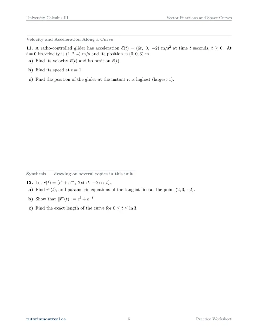
    A radio-controlled glider has acceleration $\overrightarrow{a}(t)=(6t,0,-2)\text{m}/{\text{s}}^2$ at time $t$ seconds, $t\ge 0$. At $t=0$ its velocity is $(1,2,4)\text{m}/\text{s}$ and its position is $(0,0,3)$ m.

    1. Find its velocity $\overrightarrow{v}(t)$ and its position $\overrightarrow{r}(t)$.
    2. Find its speed at $t=1$.
    3. Find the position of the glider at the instant it is highest (largest $z$).
12. Q12Synthesis — drawing on several topics in this unit

    Let $\overrightarrow{r}(t)=(e^t+e^{-t},2\sin t,-2\cos t)$.

    1. Find $\overrightarrow{r}{}^{\prime }(t)$, and parametric equations of the tangent line at the point $(2,0,-2)$.
    2. Show that $\Vert \overrightarrow{r}{}^{\prime }(t)\Vert =e^t+e^{-t}$.
    3. Find the exact length of the curve for $0\le t\le \ln 3$.

The 9 challenge problems for this topic are a separate, paid sheet and are not reproduced here.

The rest of this unit

The worksheet is the practice, and it is free. Two more printable documents cover the same unit and come with the University Calculus III bundle: read the notes first, work this sheet, then sit the test closed-book. See what each one covers.

What the Vector Functions and Space Curves notes cover  About the Vector Functions and Space Curves unit test

How to do every concept on this sheet

This is the part worksheet sites usually leave out. Below is the actual reasoning behind each group of questions — not a full solution set, the decisions that get you to one. Read it before you start, or after you get stuck.

A parametric curve is its formulas and its interval

Q1 gives a plane curve as two formulas in t with t restricted to an interval, and asks for three things that look routine: a Cartesian equation, a sketch with a direction arrow, and the points where the curve crosses the y-axis. Eliminating the parameter is the easy half — solve the linear formula for t and substitute into the other — and the result is a familiar curve you should be able to name on sight.

For the direction arrow, look at whichever coordinate changes monotonically with t: it tells you which way the curve is traced without plotting a single intermediate point, and it is what distinguishes the curve drawn by this parametrization from the same set of points traced the other way.

Where two surfaces meet: let the simpler one choose the parameter

Q2 is the other direction: a cylinder and a plane cut out a closed curve, and you have to produce its parametric equations. The method is to parametrize whichever surface already constrains two coordinates on its own, then let the other surface supply the third.

A vector function is defined where every component is

Q3 has three components of three different kinds — a logarithm, a square root and a quotient — and part (a) asks for the domain of the whole vector function. Each component brings its own restriction, and the domain of the vector function is the intersection of the three, because a vector with one undefined entry is not a vector at all.

Part (b) asks for a limit and the reason the method is valid. The limit of a vector function is the vector of the component limits, and at a point inside the domain where every component is continuous, substitution is legitimate. Saying so — continuity of each component at that point — is the justification the question wants.

When substitution fails, it fails one component at a time

Q4 is built so that direct substitution fails in two components for two different reasons and works in the third. Treat it as three separate one-variable limits and choose the tool each one needs.

Part (b) is the continuity condition from Calculus I, promoted to vectors: a vector function is continuous at a point when its value there equals its limit there. The value to assign is therefore not a new calculation — it is the answer to part (a), stated as a value.

Differentiate and integrate one component at a time

Q5 asks for r′(t), then r′(0), then a unit tangent vector at t = 0. The derivative is taken component by component with the ordinary rules — here a product rule in one component and a chain rule in the other two — so the calculus is Calculus I. What is new is what the result means: r′(t) points along the curve, in the direction of increasing t.

Q6 runs the other way: a definite integral of a vector function over an interval. It is three definite integrals, and the answer is a vector. Each component is a technique you already own — look at each integrand and decide between integration by parts, a substitution that the numerator is set up for, and an antiderivative you should recognise on sight. The question asks for an exact answer, so leave logarithms and multiples of π as they are.

A tangent line starts by finding t

Q7 gives the curve and a point on it, and asks for the tangent line there. The point is given in coordinates, but the derivative is a function of t, so the first job is to find the value of t at which the curve passes through that point.

With t in hand the rest is a line in space from CEGEP Linear Algebra: the point is the position, the direction vector is r′ at that t. Use a fresh letter for the line's own parameter, because the line's parameter and the curve's are different quantities and reusing t invites substituting one into the other.

Arc length: the integrand is designed to simplify

The formula is the easy part; the square root is the whole problem. A square root of a sum of squares has no antiderivative in general, so a worksheet question is always built so that the expression under the root collapses. Q8 and Q9 show the two ways it does.

Curvature: find t, then r′ and r″ at that t

Q10 states the formula and asks for the curvature at a given point:

The order of work matters more than the formula. As in Q7, the point is given in coordinates, so first find the t that produces it and check it in all three components. Then evaluate r′ and r″ at that t — two vectors of numbers — and only then take the cross product. Crossing the symbolic derivatives first is legal and multiplies the algebra several times over.

From acceleration back to position

Q11 gives a glider's acceleration as a function of time and its velocity and position at t = 0, and asks for the velocity and position functions, the speed at one instant, and where the glider is when it is highest. Integrating a vector function is component by component, and each integration produces a constant vector, not a single constant.

The synthesis question, and why it is last

Q12 draws on three of the sheets at once. Part (a) is a derivative and a tangent line, and the point is again given in coordinates: find the t that produces it first, as in Q7. Part (b) asks you to show a formula for the speed, so the expansion has to be written out: square each component of r′, let the two trigonometric terms combine as they did in Q8, and recognise the remaining exponential terms as a perfect square, as in Q9. Part (c) is then an arc-length integral whose integrand part (b) has already simplified, over an interval with a logarithm at one end, so simplify expressions like e raised to a logarithm before you evaluate anything.

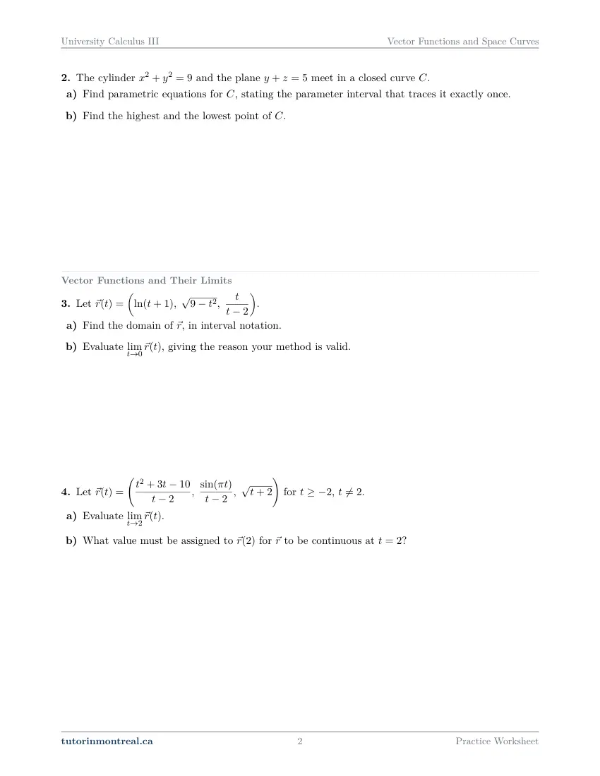
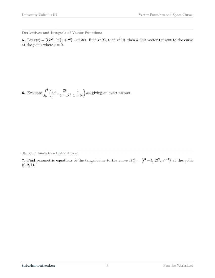
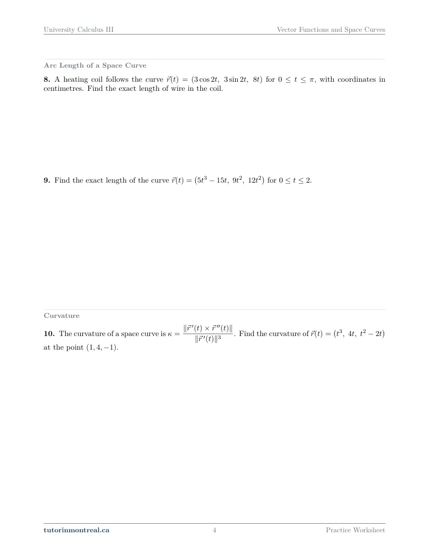
Preview all 6 pages

Click any page to open the full PDF.

Getting the most out of it

Find the parameter before you differentiate

A tangent line, a unit tangent vector or a curvature "at the point (x, y, z)" always needs the value of t first, and three of the questions here hinge on it. Solve the simplest component equation, then check the value in the other two. It is one line, and skipping it is how a correct computation gets done at the wrong point.

Say "component by component" and mean it

Domains, limits, continuity, derivatives and integrals of a vector function are all one-variable problems run three times. Lay the work out in three labelled lines rather than as one long vector expression; it keeps the techniques separate when each component needs a different one, and it makes the error easy to find when one does go wrong.

Evaluate early, cross late

Whenever a question asks about one point — a unit tangent, a curvature — substitute the value of t into r′ and r″ before normalising or crossing. Vectors of numbers are quicker and far safer than symbolic vectors, and the cross product in particular rewards it.

Check against geometry

Every answer in this set has a cheap sanity check: substitute a parametrization back into the surfaces it came from; dot a cross product with its factors; compare an arc length with the chord between its endpoints; confirm a highest point really is a maximum. Build the habit of writing one check per question, and most of the errors that cost marks never reach the page.

Common questions