University Differential Equations — Differential Equations and Direction Fields Worksheet

8 of the 10 questions

Each question targets one named concept from the sheet. Read them here, or print the PDF — it has working space under each one. 8 of the 10 questions are printed below. The other 2 are built on a diagram or a table of values that does not translate to the page, so they are in the free PDF — marked below where they would have come.

1. Q1Order, Linearity and Classification of an Equation

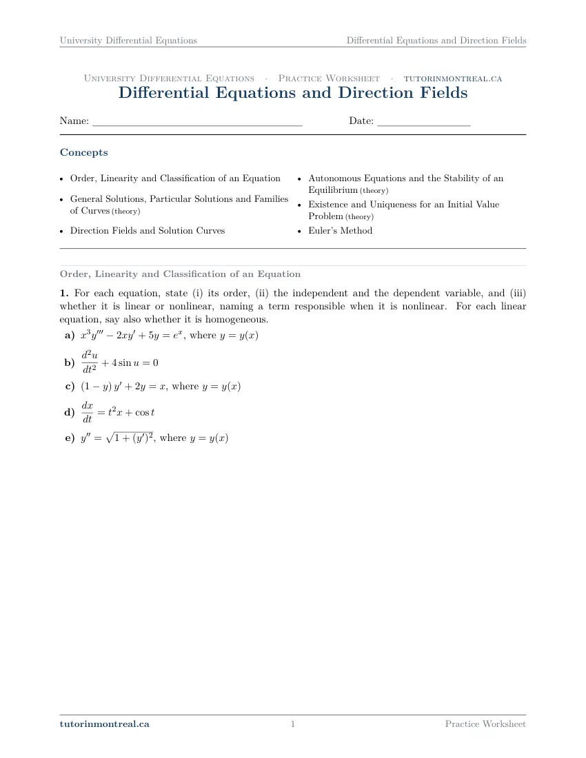
   For each equation, state (i) its order, (ii) the independent and the dependent variable, and (iii) whether it is linear or nonlinear, naming a term responsible when it is nonlinear. For each linear equation, say also whether it is homogeneous.

   1. $x^3{y}^{‴}-2x{y}^{\prime }+5y=e^x$, where $y=y(x)$
   2. ${\displaystyle \frac{d^{2}u}{d{t}^2}}+4\sin u=0$
   3. $(1-y)y^{\prime }+2y=x$, where $y=y(x)$
   4. ${\displaystyle \frac{dx}{dt}}=t^{2}x+\cos t$
   5. $y^{″}=\sqrt{1+(y^{\prime }{)}^2}$, where $y=y(x)$
2. Q2Order, Linearity and Classification of an Equation

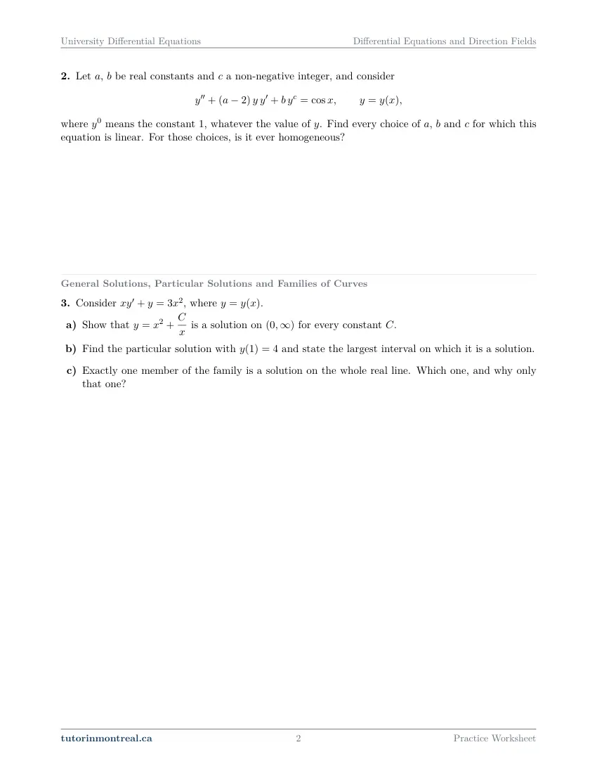
   Let $a$, $b$ be real constants and $c$ a non-negative integer, and consider $$y^{″}+(a-2)y{y}^{\prime }+b{y}^c=\cos x,y=y(x),$$ where $y^0$ means the constant $1$, whatever the value of $y$. Find every choice of $a$, $b$ and $c$ for which this equation is linear. For those choices, is it ever homogeneous?

3. Q3General Solutions, Particular Solutions and Families of Curves

   Consider $x{y}^{\prime }+y=3x^2$, where $y=y(x)$.

   1. Show that $y=x^2+{\displaystyle \frac{C}{x}}$ is a solution on $(0,\infty )$ for every constant $C$.
   2. Find the particular solution with $y(1)=4$ and state the largest interval on which it is a solution.
   3. Exactly one member of the family is a solution on the whole real line. Which one, and why only that one?
4. Q4Direction Fields and Solution Curves

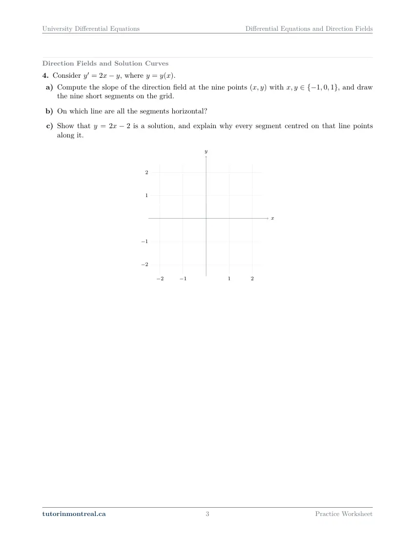
   This question is built around a diagram or a table of values. Open it in the PDF.

5. Q5Direction Fields and Solution Curves

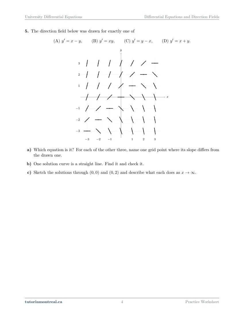
   This question is built around a diagram or a table of values. Open it in the PDF.

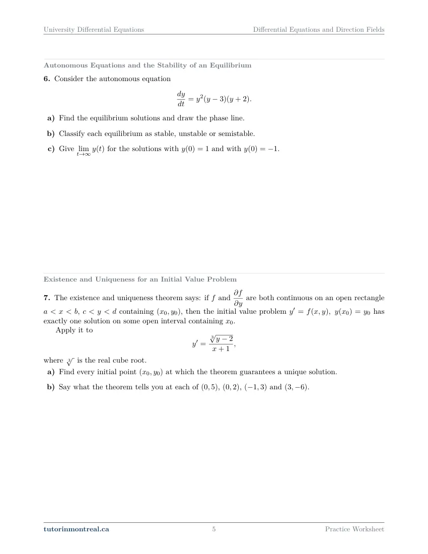
6. Q6Autonomous Equations and the Stability of an Equilibrium

   Consider the autonomous equation $$\frac{dy}{dt}=y^2(y-3)(y+2).$$

   1. Find the equilibrium solutions and draw the phase line.
   2. Classify each equilibrium as stable, unstable or semistable.
   3. Give ${\displaystyle {lim}_{t\to \infty }y(t)}$ for the solutions with $y(0)=1$ and with $y(0)=-1$.
7. Q7Existence and Uniqueness for an Initial Value Problem

   The existence and uniqueness theorem says: if $f$ and ${\displaystyle \frac{\partial f}{\partial y}}$ are both continuous on an open rectangle $a<x<b$, $c<y<d$ containing $(x_0,y_0)$, then the initial value problem $y^{\prime }=f(x,y),y(x_0)=y_0$ has exactly one solution on some open interval containing $x_0$.

   Apply it to $$y^{\prime }=\frac{\sqrt[3]{y-2}}{x+1},$$ where $\sqrt[3]{}$ is the real cube root.

   1. Find every initial point $(x_0,y_0)$ at which the theorem guarantees a unique solution.
   2. Say what the theorem tells you at each of $(0,5)$, $(0,2)$, $(-1,3)$ and $(3,-6)$.
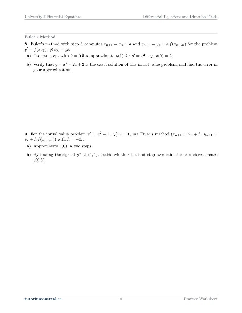
8. Q8Euler's Method

   Euler's method with step $h$ computes $x_{n+1}=x_n+h$ and $y_{n+1}=y_n+hf(x_n,y_n)$ for the problem $y^{\prime }=f(x,y),y(x_0)=y_0$.

   1. Use two steps with $h=0.5$ to approximate $y(1)$ for $y^{\prime }=x^2-y,y(0)=2$.
   2. Verify that $y=x^2-2x+2$ is the exact solution of this initial value problem, and find the error in your approximation.
9. Q9Euler's Method

   For the initial value problem $y^{\prime }=y^2-x,y(1)=1$, use Euler's method ($x_{n+1}=x_n+h$, $y_{n+1}=y_n+hf(x_n,y_n)$) with $h=-0.5$.

   1. Approximate $y(0)$ in two steps.
   2. By finding the sign of $y^{″}$ at $(1,1)$, decide whether the first step overestimates or underestimates $y(0.5)$.
10. Q10Synthesis — drawing on several topics in this unit

    The existence and uniqueness theorem says: if $f$ and ${\displaystyle \frac{\partial f}{\partial y}}$ are both continuous on an open rectangle containing $(x_0,y_0)$, then $y^{\prime }=f(x,y),y(x_0)=y_0$ has exactly one solution on some open interval containing $x_0$. Consider $$x{y}^{\prime }=2y,y=y(x).$$

    1. State its order and whether it is linear and homogeneous.
    2. Show that $y=C{x}^2$ is a solution on all of $ℝ$ for every constant $C$.
    3. Show that no solution has $y(0)=1$, and that infinitely many have $y(0)=0$.
    4. Explain why (c) does not contradict the theorem, and say at which points $(x_0,y_0)$ the theorem does guarantee a unique solution.

The 7 challenge problems for this topic are a separate, paid sheet and are not reproduced here.

How to do every concept on this sheet

This is the part worksheet sites usually leave out. Below is the actual reasoning behind each group of questions — not a full solution set, the decisions that get you to one. Read it before you start, or after you get stuck.

Order, linearity and homogeneity

The order of an equation is the order of the highest derivative in it — not the highest power. An equation in y(x) is linear when it can be written as a sum of terms, each of which is y or one of its derivatives multiplied by a function of x alone, set equal to a function of x alone. Q1 asks for all three labels on five equations, and for a nonlinear one it asks you to point at the term that breaks linearity.

Q2 turns the test into a parameter problem. Look at each term containing y in turn and ask which values of the parameters make that term either disappear or become linear. The convention that y⁰ means the constant 1 matters: a term that becomes a constant is no longer a term in y at all, and belongs on the right-hand side — which is exactly what the last part, about homogeneity, is probing.

General solutions, particular solutions, and where they live

A one-parameter family such as y = x² + C/x is a general solution of a first-order equation; fixing the constant with an initial condition picks out one particular solution. Q3(a) is a verification: differentiate the family and substitute into the equation, keeping C as a letter.

Q3(c) asks which member survives on the whole real line. Look at what the troublesome term needs in order to disappear, and explain why no other choice of the constant can repair the problem at that point.

Direction fields

For y′ = f(x, y), the equation hands you the slope of the solution through every point without solving anything. A direction field draws a short segment of that slope at each grid point, and a solution curve is any curve that runs tangent to the segments everywhere. Q4(a) is the construction by hand at nine points.

Q4(b) asks where the segments are horizontal: that is where f(x, y) = 0, a curve called a nullcline or isocline of slope zero. Q4(c) shows a line that is itself a solution. Substitute it to check, and then explain the geometry: a segment drawn on a solution curve has the same slope as the curve, so it lies along it.

Q5 runs the reading the other way. Four candidate equations, one drawn field: choose a few easy grid points — on the axes, or on a diagonal — compute each candidate's slope there, and compare with the drawing. One disagreement is enough to eliminate a candidate, and Q5(a) asks you to name one for each. Part (b) looks for a straight-line solution: try y = mx + b, and require the slope m to equal f along the whole line. Part (c) is sketching — follow the segments from each starting point and say what the curve approaches.

Autonomous equations and the phase line

An autonomous equation has the form dy/dt = g(y): the slope does not depend on t. Its equilibria are the constant solutions, the zeros of g. Between them, the sign of g says whether y rises or falls, and that is all the phase line records. Q6 builds one.

Q6(c) asks for long-run behaviour. A solution starts between two equilibria, can never cross either (uniqueness forbids it), and moves in the direction of the arrow — so it tends to the equilibrium the arrow points at.

Existence and uniqueness

Q7 states the theorem and asks you to apply it. The work is identifying where f and ∂f/∂y are continuous. Write f(x, y) out, differentiate it with respect to y, and list the places where either one fails: a denominator that vanishes, a root of something that becomes zero where the derivative of the root blows up.

Q7(b) contains a point on each of the problem lines and points away from them; the answer for each is a sentence about the hypotheses, not a solution.

Euler's method

Euler's method walks along the direction field: from the current point, follow the tangent line for one step of length h, then recompute the slope at the new point. Q8 and Q9 give the formulas.

Q8(a) is two forward steps; lay the work out as a table with columns n, xₙ, yₙ and f(xₙ, yₙ) so that each row feeds the next. Q8(b) verifies an exact solution by substitution and checking the initial condition, then compares: the error is the exact value minus the approximation.

Q9 steps backwards. A negative h is perfectly legal — the formula is the same, and xₙ decreases. Part (b) asks whether the first step over- or underestimates. Differentiate y′ = f(x, y) implicitly to get y″ in terms of x, y and y′, evaluate it at the starting point, and use concavity: a tangent line lies above a concave-down curve and below a concave-up one.

The synthesis question

Q10 puts the set together on one equation. Part (a) is Q1. Part (b) is Q3(a), with the extra demand that the solution hold on all of the real line — including the point where the equation's leading coefficient vanishes. Part (c) asks you to prove two things about the initial point at x = 0 using the family from (b): substitute x = 0 into the equation itself to see what any solution must satisfy there. Part (d) is Q7: write the equation as y′ = f(x, y), find where the hypotheses fail, and explain why part (c) is not a contradiction — the theorem said nothing at those points.

Preview all 7 pages

Click any page to open the full PDF.

Getting the most out of it

Classify before you do anything else

Order, linearity and whether an equation is autonomous decide which tools apply. Write the three labels down at the start of every question; it takes a few seconds and it is what the rest of the course asks first.

Draw the picture

A handful of segments or a phase line often answers a question about long-run behaviour with no solving at all. When a question says "describe", it usually wants the picture read aloud.

Quote the hypothesis you are checking

For existence and uniqueness, write f and ∂f/∂y explicitly and say where each is continuous. "The theorem applies" without that is not an answer.

Tabulate Euler steps

One row per step, with the slope in its own column. Most errors in Euler's method are a slope evaluated at the wrong point, and a table makes that visible.

Common questions