University Differential Equations — First-Order Solution Methods Worksheet

All 12 questions

Each question targets one named concept from the sheet. Read them here, or print the PDF — it has working space under each one.

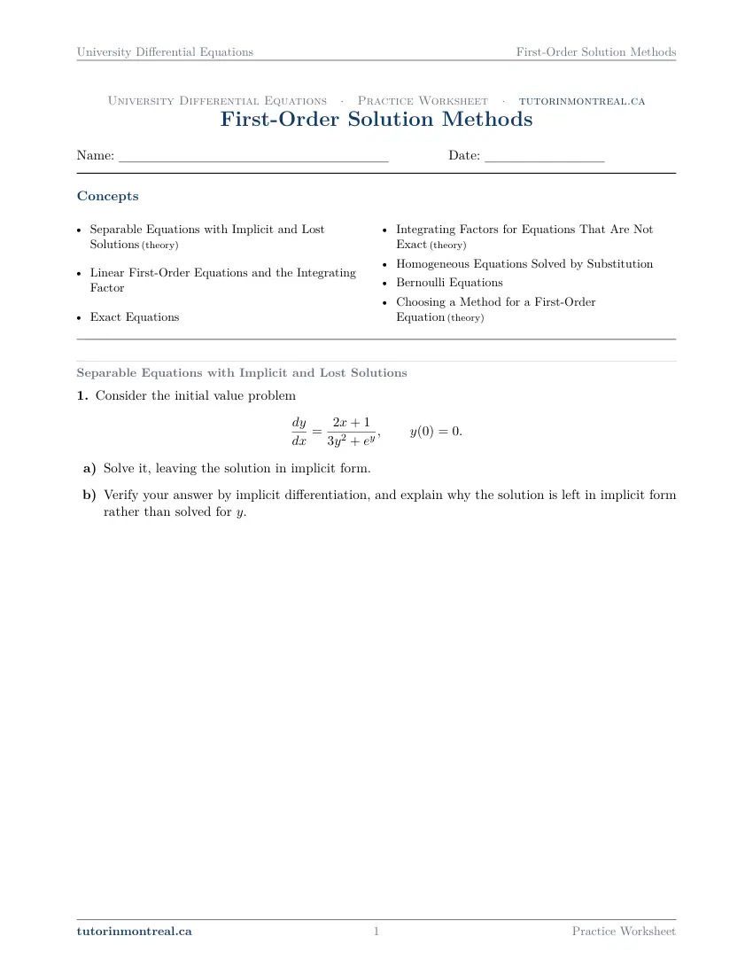
1. Q1Separable Equations with Implicit and Lost Solutions

   Consider the initial value problem $$\frac{dy}{dx}=\frac{2x+1}{3y^2+e^y},y(0)=0.$$

   1. Solve it, leaving the solution in implicit form.
   2. Verify your answer by implicit differentiation, and explain why the solution is left in implicit form rather than solved for $y$.
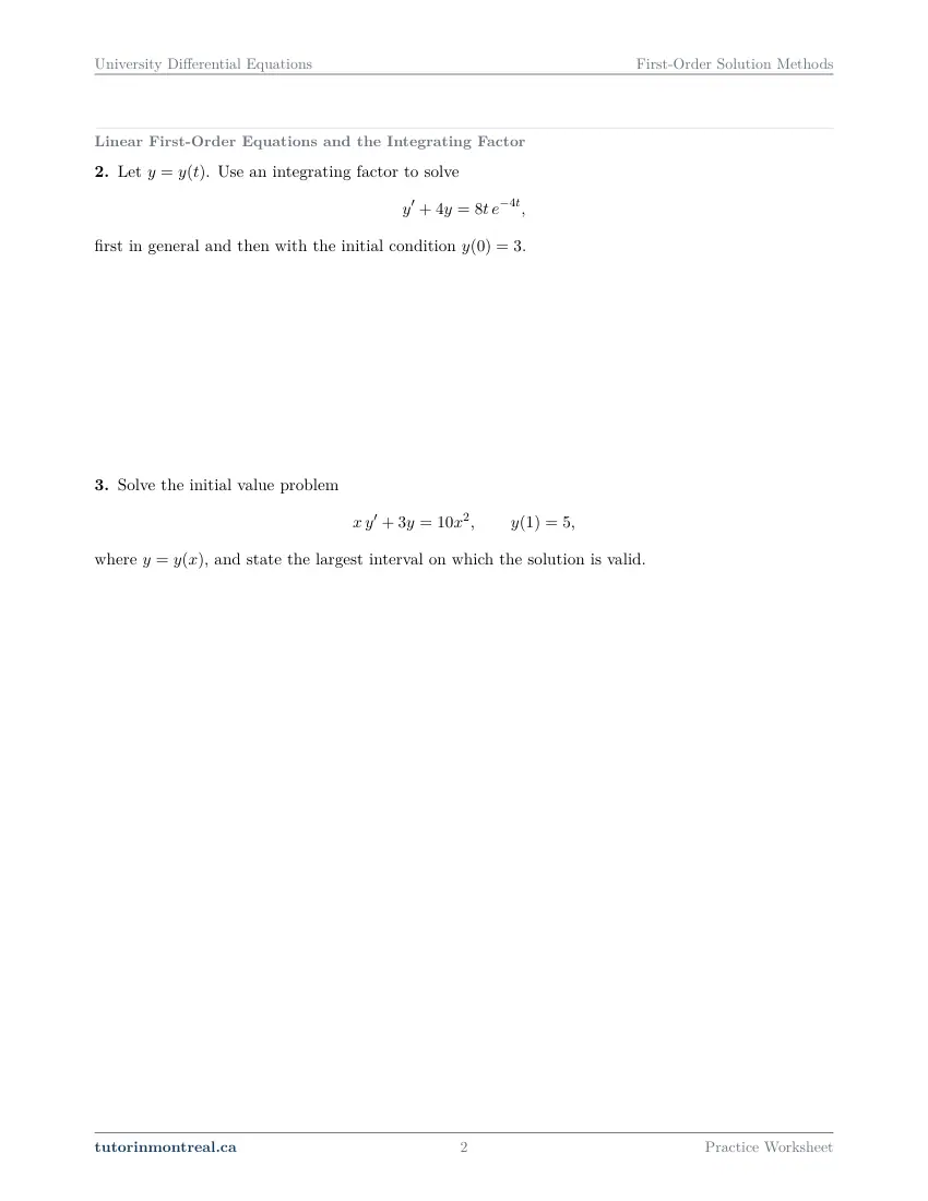
2. Q2Linear First-Order Equations and the Integrating Factor

   Let $y=y(t)$. Use an integrating factor to solve $$y^{\prime }+4y=8t{e}^{-4t},$$ first in general and then with the initial condition $y(0)=3$.

3. Q3Linear First-Order Equations and the Integrating Factor

   Solve the initial value problem $$x{y}^{\prime }+3y=10x^2,y(1)=5,$$ where $y=y(x)$, and state the largest interval on which the solution is valid.

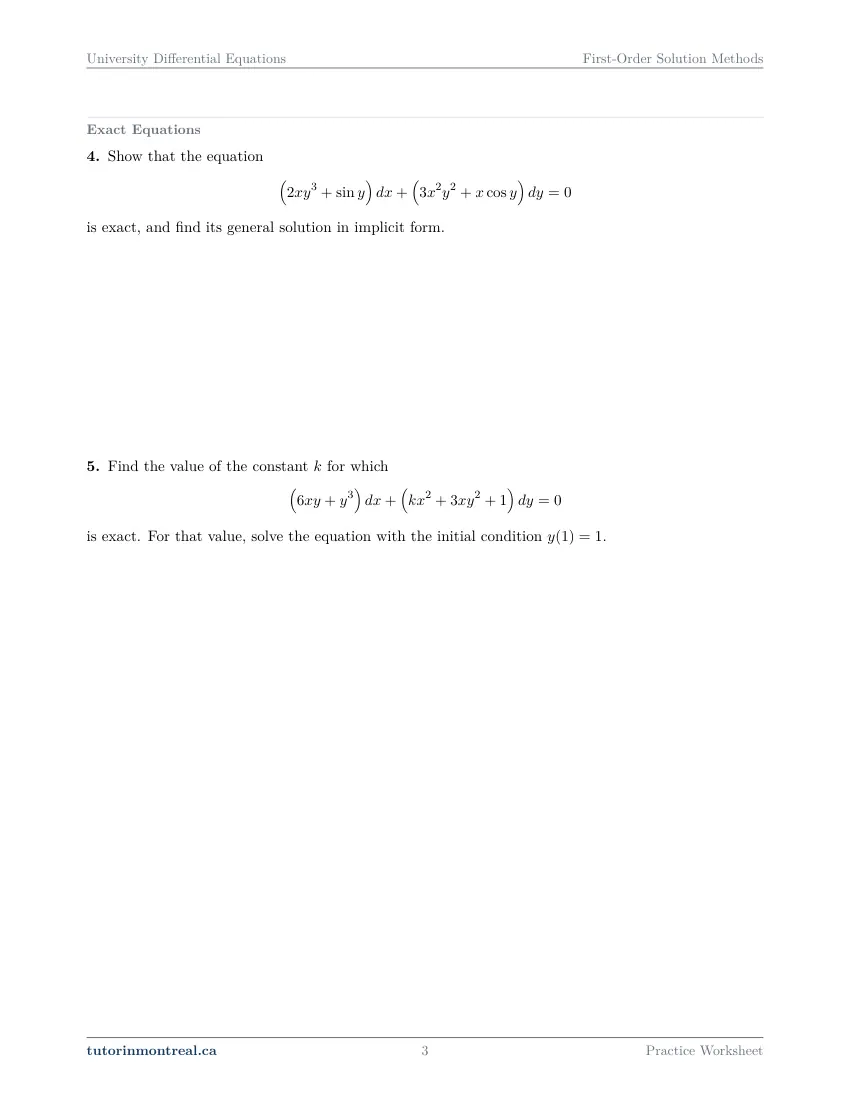
4. Q4Exact Equations

   Show that the equation $$(2x{y}^3+\sin y)dx+(3x^2{y}^2+x\cos y)dy=0$$ is exact, and find its general solution in implicit form.

5. Q5Exact Equations

   Find the value of the constant $k$ for which $$(6xy+y^3)dx+(k{x}^2+3x{y}^2+1)dy=0$$ is exact. For that value, solve the equation with the initial condition $y(1)=1$.

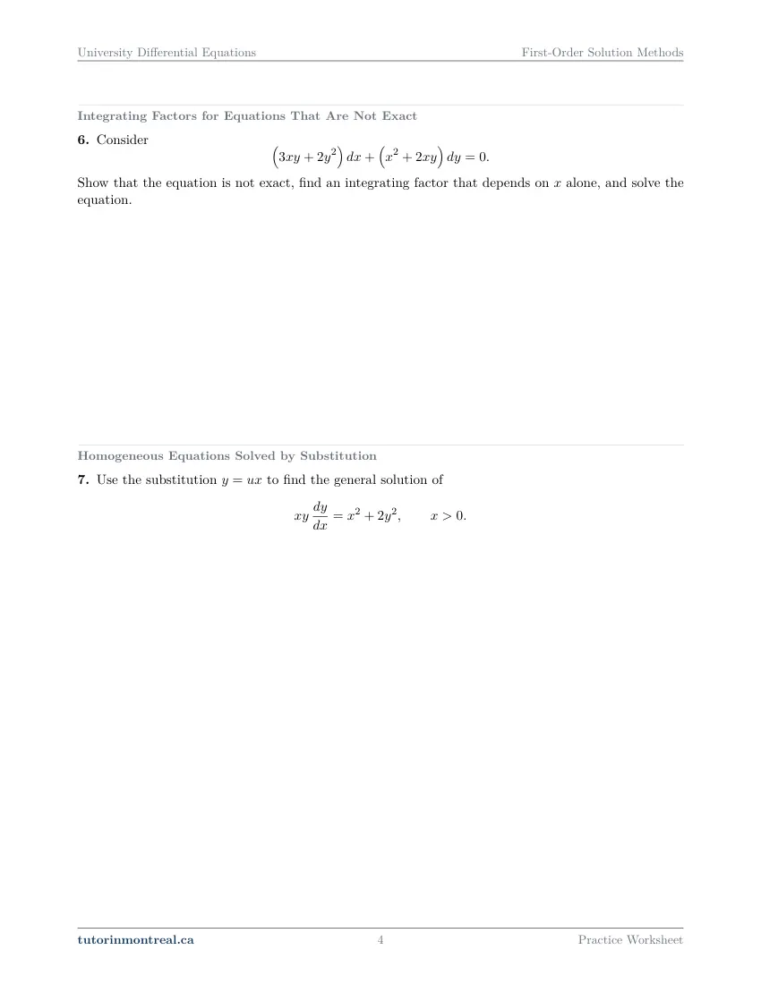
6. Q6Integrating Factors for Equations That Are Not Exact

   Consider $$(3xy+2y^2)dx+(x^2+2xy)dy=0.$$ Show that the equation is not exact, find an integrating factor that depends on $x$ alone, and solve the equation.

7. Q7Homogeneous Equations Solved by Substitution

   Use the substitution $y=ux$ to find the general solution of $$xy\frac{dy}{dx}=x^2+2y^2,x>0.$$

8. Q8Homogeneous Equations Solved by Substitution

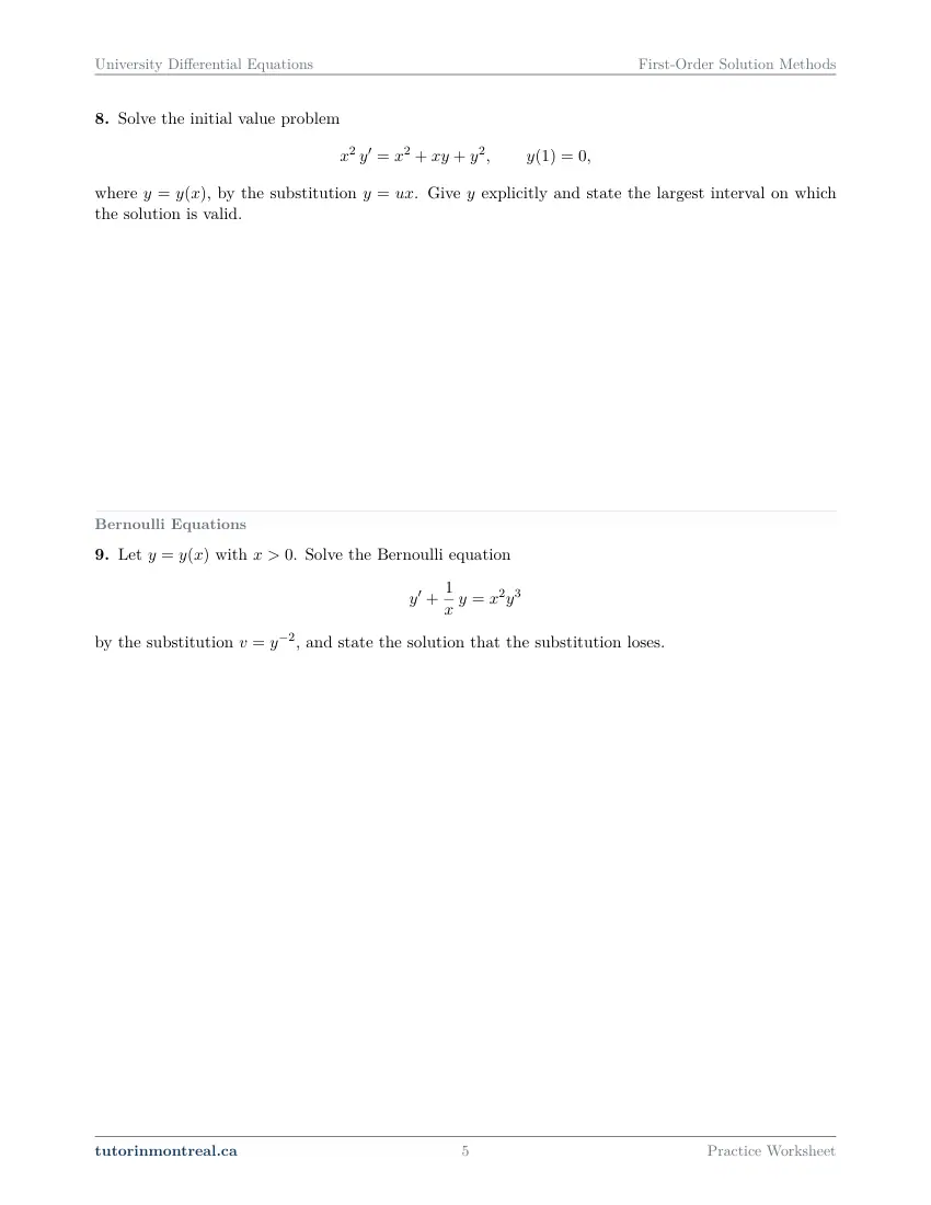
   Solve the initial value problem $$x^2{y}^{\prime }=x^2+xy+y^2,y(1)=0,$$ where $y=y(x)$, by the substitution $y=ux$. Give $y$ explicitly and state the largest interval on which the solution is valid.

9. Q9Bernoulli Equations

   Let $y=y(x)$ with $x>0$. Solve the Bernoulli equation $$y^{\prime }+\frac{1}{x}y=x^2{y}^3$$ by the substitution $v=y^{-2}$, and state the solution that the substitution loses.

10. Q10Bernoulli Equations

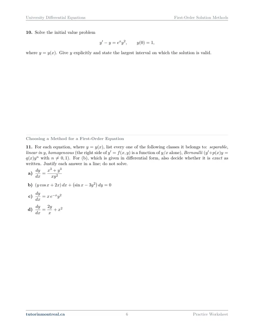
    Solve the initial value problem $$y^{\prime }-y=e^x{y}^2,y(0)=1,$$ where $y=y(x)$. Give $y$ explicitly and state the largest interval on which the solution is valid.

11. Q11Choosing a Method for a First-Order Equation

    For each equation, where $y=y(x)$, list every one of the following classes it belongs to: separable, linear in $y$, homogeneous (the right side of $y^{\prime }=f(x,y)$ is a function of $y/x$ alone), Bernoulli ($y^{\prime }+p(x)y=q(x)y^n$ with $n\ne 0,1$). For (b), which is given in differential form, also decide whether it is exact as written. Justify each answer in a line; do not solve.

    1. ${\displaystyle \frac{dy}{dx}}={\displaystyle \frac{x^3+y^3}{x{y}^2}}$
    2. $(y\cos x+2x)dx+(\sin x-3y^2)dy=0$
    3. ${\displaystyle \frac{dy}{dx}}=x{e}^{-x}{y}^2$
    4. ${\displaystyle \frac{dy}{dx}}={\displaystyle \frac{2y}{x}}+x^2$
12. Q12Synthesis — drawing on several topics in this unit

    Consider the initial value problem $$2xy{y}^{\prime }=3y^2-x^2,y(1)=2,$$ where $y=y(x)$ and $x>0$.

    1. Solve it by the substitution $y=ux$.
    2. Solve it again as a Bernoulli equation, with the substitution $v=y^2$, and confirm that the two answers agree.
    3. Give $y$ explicitly and state its interval of validity.

The 8 challenge problems for this topic are a separate, paid sheet and are not reproduced here.

How to do every concept on this sheet

This is the part worksheet sites usually leave out. Below is the actual reasoning behind each group of questions — not a full solution set, the decisions that get you to one. Read it before you start, or after you get stuck.

Separable equations, left implicit

CEGEP Calculus II separates and integrates. Q1 adds what that course leaves out: an equation whose integrated form cannot be solved for y. Separate the variables so that every y is with dy and every x with dx, integrate both sides, and use the initial condition to fix the constant while the relation is still implicit.

Linear equations and the integrating factor

A first-order linear equation can always be put in standard form, y′ + P(x)y = Q(x). Multiplying by μ = e^(∫P dx) turns the left side into the derivative of a product, and one integration finishes the job.

Q2 is the method in its cleanest form, with the variable t: watch what the factor does to the exponential on the right. Q3 needs step 1 first — the coefficient of y′ is x — and then asks for the interval of validity. Dividing by x is exactly what makes x = 0 a boundary, so the interval is the one that contains the initial point and stops there.

Exact equations

An equation M dx + N dy = 0 is exact when it is the total differential of some function F(x, y), and then the solution is F(x, y) = C. The test is equality of mixed partials.

Q4 asks you to show exactness first — compute both partials and write them side by side — and then recover F. Q5 reverses the order: the exactness condition is an equation for the unknown constant k. Solve it, then solve the exact equation and apply the initial condition to the implicit solution.

Integrating factors for equations that are not exact

Q6 gives an equation that fails the test and asks for a factor that depends on x alone. Multiplying by μ(x) and demanding exactness gives a condition that only works out when a certain quotient depends on x alone.

Compute the quotient, check that every y cancels (if it does not, a factor in x alone does not exist), build μ, multiply the whole equation through, and confirm exactness again before recovering F. That last check costs one line and catches an arithmetic slip in μ.

Homogeneous equations: the substitution y = ux

An equation is homogeneous in this sense when y′ can be written as a function of y/x alone. The substitution y = ux, with y′ = u + xu′, turns it into a separable equation in u and x. Q7 and Q8 both name the substitution.

Q8 asks for y explicitly and for the largest interval of validity. When the u-integral produces an inverse trigonometric function, solving for y means applying the trigonometric function — and that function has asymptotes, which set the ends of the interval together with x > 0.

Bernoulli equations

y′ + P(x)y = Q(x)yⁿ is linear except for the power n. The substitution v = y¹⁻ⁿ makes it linear in v, and then the integrating factor finishes it.

Divide the equation by yⁿ first, then replace y¹⁻ⁿ by v and y⁻ⁿy′ by v′/(1 − n). In Q9 the substitution is named for you. Its last demand is the lost solution: dividing by yⁿ assumed y was never zero, so ask whether the function that is zero everywhere solves the original equation.

Q10 leaves the substitution to you: identify n, write v, and solve the linear equation in v with the initial condition transferred to v. Then solve back for y and find where the expression breaks down — a denominator that can reach zero is what ends the interval.

Choosing a method

Q11 asks for classification only, with a one-line reason for each label. An equation can belong to several classes, and the question wants every one. Put each equation in the form y′ = f(x, y) and test the definitions directly.

A justification is a line of algebra, not a verdict: show the factorisation, the rescaling, or the rearrangement that matches the form.

The synthesis question

Q12 solves one initial value problem two ways. Part (a) is Q7's substitution; part (b) rearranges the same equation into a Bernoulli equation and uses the substitution it names. Agreement between the two is the check. Part (c) is Q8 and Q10: an explicit y, and an interval set by x > 0 and by wherever the expression under a root or in a denominator stops being allowed.

Preview all 7 pages

Click any page to open the full PDF.

Getting the most out of it

Classify first, then solve

Before any algebra, write down which classes the equation belongs to. The Q11 habit — one line of justification per class — is what an exam question saying "solve" silently expects.

Write the form you are matching

Standard linear form, M dx + N dy = 0, y′ = f(y/x), y′ + Py = Qyⁿ: write the template above your work and line the equation up under it. Most method errors are a coefficient read off the wrong form.

Check every solution

Differentiate your answer, implicitly if you must, and substitute. It is the only check that catches a lost constant, a wrong integrating factor and a sign error at once.

Hunt for lost solutions and state the interval

Every division by an expression in y can lose a solution, and every division by an expression in x can end an interval. Make both checks part of finishing a question.

Common questions