University Differential Equations — Power Series Solutions Worksheet

All 7 questions

Each question targets one named concept from the sheet. Read them here, or print the PDF — it has working space under each one.

1. Q1Shifting the Index of Summation

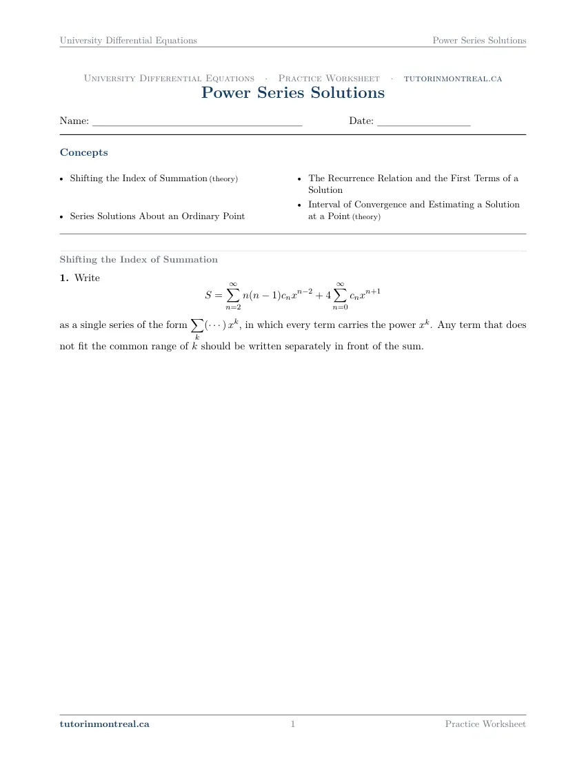
   Write $$S={\sum }_{n=2}^{\infty }n(n-1)c_n{x}^{n-2}+4{\sum }_{n=0}^{\infty }{c}_n{x}^{n+1}$$ as a single series of the form ${\displaystyle {\sum }_k(\cdots )x^k}$, in which every term carries the power $x^k$. Any term that does not fit the common range of $k$ should be written separately in front of the sum.

2. Q2Series Solutions About an Ordinary Point

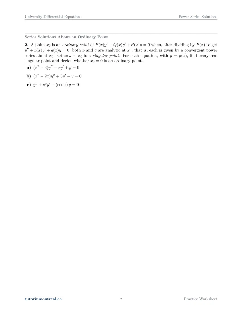
   A point $x_0$ is an ordinary point of $P(x)y^{″}+Q(x)y^{\prime }+R(x)y=0$ when, after dividing by $P(x)$ to get $y^{″}+p(x)y^{\prime }+q(x)y=0$, both $p$ and $q$ are analytic at $x_0$, that is, each is given by a convergent power series about $x_0$. Otherwise $x_0$ is a singular point. For each equation, with $y=y(x)$, find every real singular point and decide whether $x_0=0$ is an ordinary point.

   1. $(x^2+3)y^{″}-x{y}^{\prime }+y=0$
   2. $(x^2-2x)y^{″}+3y^{\prime }-y=0$
   3. $y^{″}+e^x{y}^{\prime }+(\cos x)y=0$
3. Q3Series Solutions About an Ordinary Point

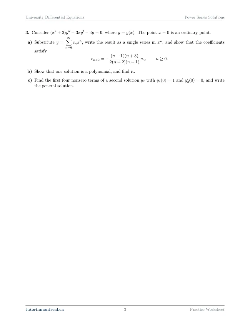
   Consider $(x^2+2)y^{″}+3x{y}^{\prime }-3y=0$, where $y=y(x)$. The point $x=0$ is an ordinary point.

   1. Substitute $y={\displaystyle {\sum }_{n=0}^{\infty }{c}_n{x}^n}$, write the result as a single series in $x^n$, and show that the coefficients satisfy $$c_{n+2}=-\frac{(n-1)(n+3)}{2(n+2)(n+1)}{c}_n,n\ge 0.$$
   2. Show that one solution is a polynomial, and find it.
   3. Find the first four nonzero terms of a second solution $y_2$ with $y_2(0)=1$ and $y_2^{\prime }(0)=0$, and write the general solution.
4. Q4The Recurrence Relation and the First Terms of a Solution

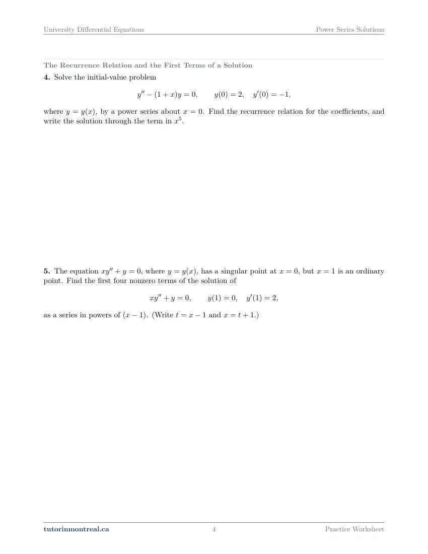
   Solve the initial-value problem $$y^{″}-(1+x)y=0,y(0)=2,y^{\prime }(0)=-1,$$ where $y=y(x)$, by a power series about $x=0$. Find the recurrence relation for the coefficients, and write the solution through the term in $x^5$.

5. Q5The Recurrence Relation and the First Terms of a Solution

   The equation $x{y}^{″}+y=0$, where $y=y(x)$, has a singular point at $x=0$, but $x=1$ is an ordinary point. Find the first four nonzero terms of the solution of $$x{y}^{″}+y=0,y(1)=0,y^{\prime }(1)=2,$$ as a series in powers of $(x-1)$. (Write $t=x-1$ and $x=t+1$.)

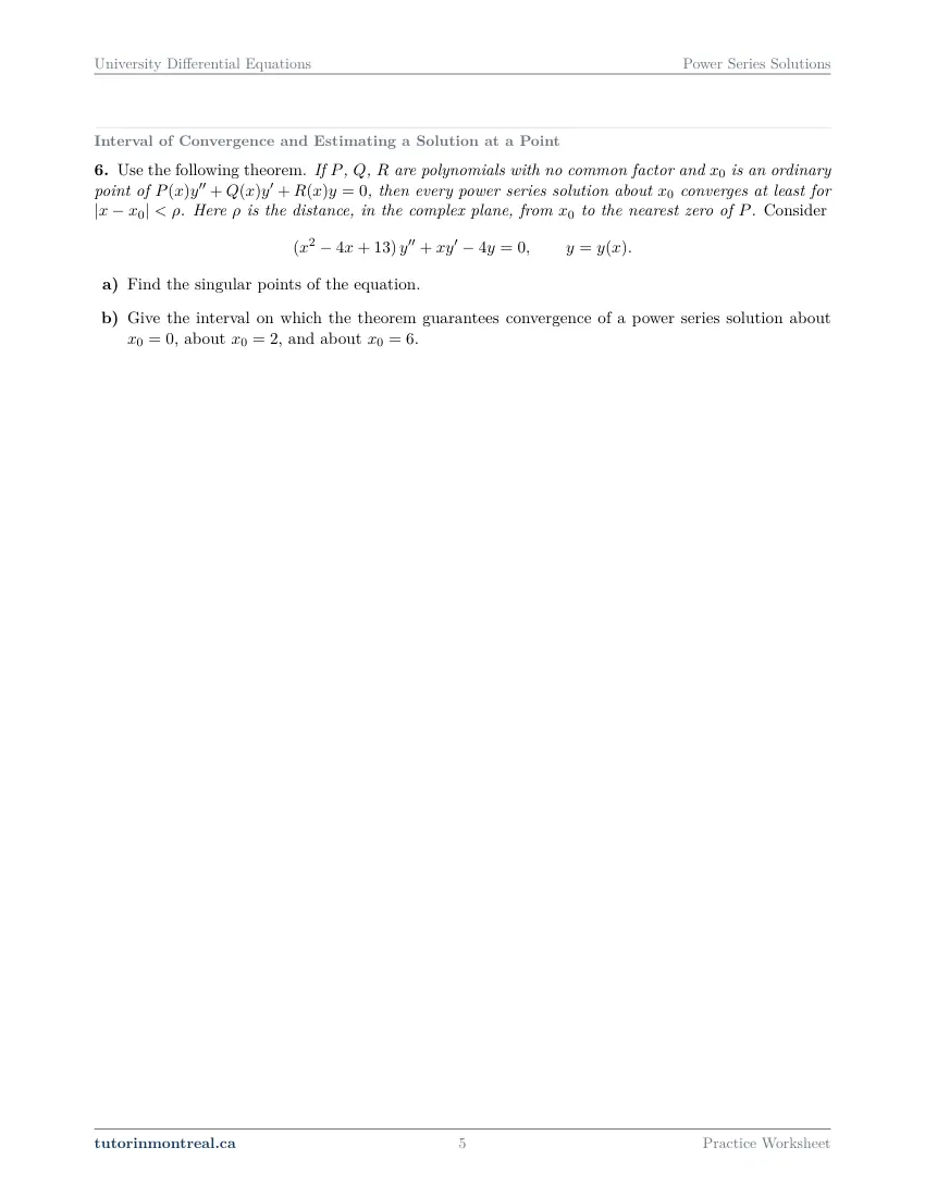
6. Q6Interval of Convergence and Estimating a Solution at a Point

   Use the following theorem. If $P$, $Q$, $R$ are polynomials with no common factor and $x_0$ is an ordinary point of $P(x)y^{″}+Q(x)y^{\prime }+R(x)y=0$, then every power series solution about $x_0$ converges at least for $|x-x_0|<\rho$. Here $\rho$ is the distance, in the complex plane, from $x_0$ to the nearest zero of $P$. Consider $$(x^2-4x+13)y^{″}+x{y}^{\prime }-4y=0,y=y(x).$$

   1. Find the singular points of the equation.
   2. Give the interval on which the theorem guarantees convergence of a power series solution about $x_0=0$, about $x_0=2$, and about $x_0=6$.
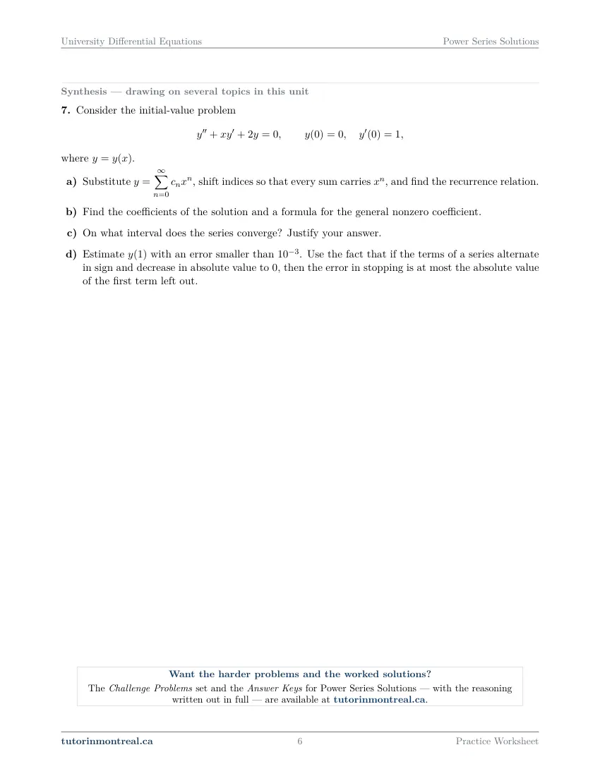
7. Q7Synthesis — drawing on several topics in this unit

   Consider the initial-value problem $$y^{″}+x{y}^{\prime }+2y=0,y(0)=0,y^{\prime }(0)=1,$$ where $y=y(x)$.

   1. Substitute $y={\displaystyle {\sum }_{n=0}^{\infty }{c}_n{x}^n}$, shift indices so that every sum carries $x^n$, and find the recurrence relation.
   2. Find the coefficients of the solution and a formula for the general nonzero coefficient.
   3. On what interval does the series converge? Justify your answer.
   4. Estimate $y(1)$ with an error smaller than ${10}^{-3}$. Use the fact that if the terms of a series alternate in sign and decrease in absolute value to $0$, then the error in stopping is at most the absolute value of the first term left out.

The 5 challenge problems for this topic are a separate, paid sheet and are not reproduced here.

How to do every concept on this sheet

This is the part worksheet sites usually leave out. Below is the actual reasoning behind each group of questions — not a full solution set, the decisions that get you to one. Read it before you start, or after you get stuck.

Shifting the index of summation

Every series solution ends with a sentence of the form "a power series is zero for every x, so each of its coefficients is zero". That sentence only applies to one series in which every term carries the same power of x. Substituting into an equation produces several series with different powers — xⁿ⁻² from y″, xⁿ⁺¹ from a term like x·y — and different starting values of n. Q1 isolates that step with no differential equation in sight.

Ordinary points and singular points

Before assuming a power series about a point, you need to know that the point is ordinary. Q2 gives the definition in full: divide by the coefficient of y″ to put the equation in the form y″ + p(x)y′ + q(x)y = 0, and ask whether p and q are both analytic at the point.

Series solutions about an ordinary point

Q3 is the method from start to finish on one equation. Part (a) assembles everything above: differentiate the assumed series twice term by term, multiply through by the coefficients — the x² and x in front of y″ and y′ change the powers, the constant does not — shift each sum to xⁿ, and set the combined coefficient equal to zero. The question tells you the recurrence you should reach, so part (a) is a check on your bookkeeping: if your version differs, find the shift that went wrong rather than forcing a match.

Part (b) asks you to show that one solution is a polynomial. The tool is the factor structure of the recurrence: look for a value of n that makes the numerator zero. Once one coefficient in a chain is zero, the recurrence forces every later coefficient in that chain to be zero, and the series stops. Say which chain it is and why nothing after that point survives. Part (c) is the other chain, with the initial conditions choosing c₀ and c₁ — write y(0) and y′(0) in terms of the coefficients before you substitute anything.

The recurrence relation and the first terms of a solution

Q4 is an initial value problem solved by series. The new feature is a coefficient with two terms. Multiplying the series for y by a sum produces two series with different powers, so after shifting, the coefficient of xⁿ involves more than two of the c's, and the lowest power is special because one of the sums has not started yet.

Q5 moves the centre. The equation is singular at x = 0 but ordinary at x = 1, and the initial conditions are given at x = 1, so the series has to be in powers of (x − 1). The question hands you the substitution: write t = x − 1, so that x = t + 1, rewrite the whole equation in t, and solve the new equation about t = 0 exactly as before.

How far the series is guaranteed to converge

Q6 states the theorem the chapter relies on: about an ordinary point, a power series solution converges at least out to the nearest zero of the leading coefficient P — measured in the complex plane, not along the real line. The radius comes from the equation, before a single coefficient has been computed.

The synthesis question

Q7 runs the whole chapter on one initial value problem. Part (a) is Q1 and Q3(a) together: substitute, shift every sum to xⁿ, read off the recurrence — here y′ is multiplied by x, which raises its power back to match the others. Part (b) is Q3's two chains with Q4's initial conditions: the two conditions fix c₀ and c₁, so decide what each one does to its chain before computing anything. Look for a pattern in the surviving coefficients and write the general one as a product; checking it against the recurrence for one more index is what turns a guess into a formula.

Part (c) is Q6's theorem, and the justification is the theorem's hypothesis and its conclusion, applied to this leading coefficient: say what P is, where its zeros are, and what that makes the guaranteed radius. Part (d) is a Calculus II estimate. Substitute x = 1 into the series, confirm that the terms alternate and decrease to zero, then keep adding terms until the first term you would leave out is smaller than the tolerance.

Preview all 6 pages

Click any page to open the full PDF.

Getting the most out of it

Write out the first term of every sum you shift

Before and after each change of index, substitute the starting value and write the first term in full. If the two do not match, the shift is wrong. It takes seconds and catches nearly every index error before it spreads into the recurrence.

Keep the low powers separate

When the sums start at different powers, write the lowest-power terms on their own line and set them equal to zero on their own. Folding them into the general recurrence by hand-waving is how a coefficient like c₂ ends up wrong, and every later coefficient in its chain inherits the error.

Tabulate the coefficients

Compute cₙ in a table, one row per n, in terms of c₀ and c₁ until you apply the initial conditions. A table makes the two chains visible, shows a zero coefficient as a zero rather than as a missing line, and makes a pattern for the general coefficient much easier to spot.

Find the radius from the equation first

Before computing any coefficient, find the zeros of the leading coefficient and the distance to the nearest one. It tells you where your series can be trusted, and it is the reason a partial sum is a legitimate estimate at the point you are asked about.

Common questions