University Differential Equations — Mechanical Vibrations and Electric Circuits Worksheet

All 10 questions

Each question targets one named concept from the sheet. Read them here, or print the PDF — it has working space under each one.

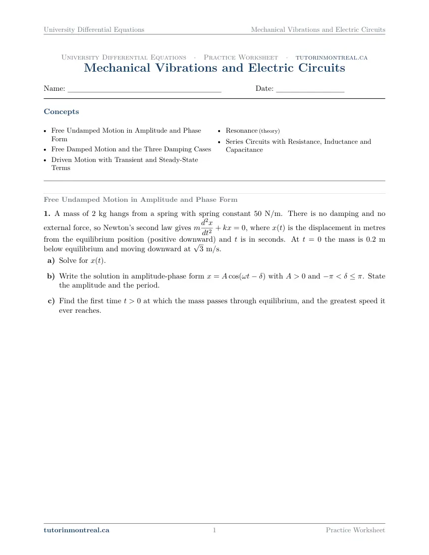
1. Q1Free Undamped Motion in Amplitude and Phase Form

   A mass of $2\text{kg}$ hangs from a spring with spring constant $50\text{N}/\text{m}$. There is no damping and no external force, so Newton's second law gives $m{\displaystyle \frac{d^{2}x}{d{t}^2}}+kx=0$, where $x(t)$ is the displacement in metres from the equilibrium position (positive downward) and $t$ is in seconds. At $t=0$ the mass is $0.2\text{m}$ below equilibrium and moving downward at $\sqrt{3}\text{m}/\text{s}$.

   1. Solve for $x(t)$.
   2. Write the solution in amplitude-phase form $x=A\cos (\omega t-\delta )$ with $A>0$ and $-\pi <\delta \le \pi$. State the amplitude and the period.
   3. Find the first time $t>0$ at which the mass passes through equilibrium, and the greatest speed it ever reaches.
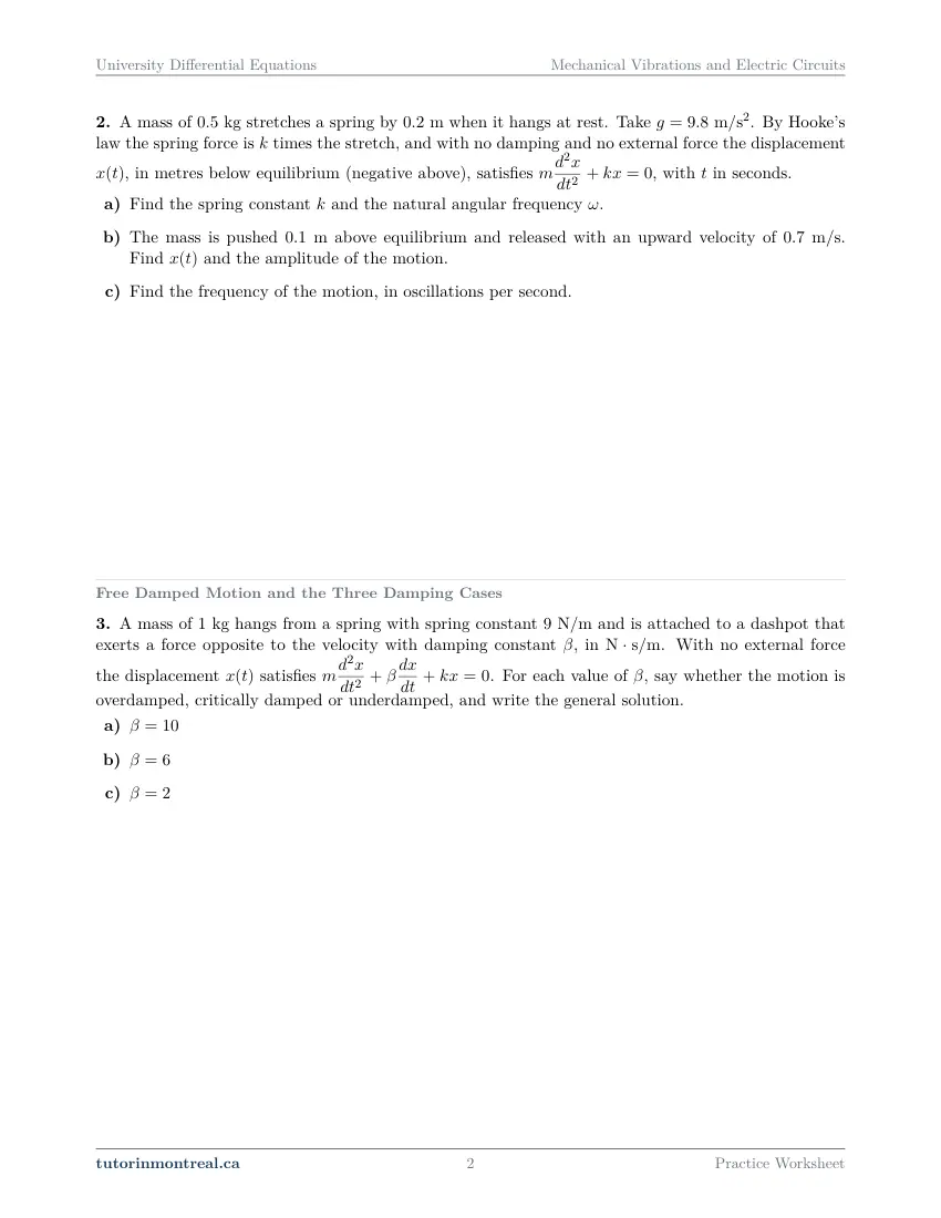
2. Q2Free Undamped Motion in Amplitude and Phase Form

   A mass of $0.5\text{kg}$ stretches a spring by $0.2\text{m}$ when it hangs at rest. Take $g=9.8\text{m}/{\text{s}}^2$. By Hooke's law the spring force is $k$ times the stretch, and with no damping and no external force the displacement $x(t)$, in metres below equilibrium (negative above), satisfies $m{\displaystyle \frac{d^{2}x}{d{t}^2}}+kx=0$, with $t$ in seconds.

   1. Find the spring constant $k$ and the natural angular frequency $\omega$.
   2. The mass is pushed $0.1\text{m}$ above equilibrium and released with an upward velocity of $0.7\text{m}/\text{s}$. Find $x(t)$ and the amplitude of the motion.
   3. Find the frequency of the motion, in oscillations per second.
3. Q3Free Damped Motion and the Three Damping Cases

   A mass of $1\text{kg}$ hangs from a spring with spring constant $9\text{N}/\text{m}$ and is attached to a dashpot that exerts a force opposite to the velocity with damping constant $\beta$, in $\text{N}·\text{s}/\text{m}$. With no external force the displacement $x(t)$ satisfies $m{\displaystyle \frac{d^{2}x}{d{t}^2}}+\beta {\displaystyle \frac{dx}{dt}}+kx=0$. For each value of $\beta$, say whether the motion is overdamped, critically damped or underdamped, and write the general solution.

   1. $\beta =10$
   2. $\beta =6$
   3. $\beta =2$
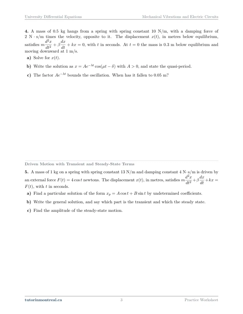
4. Q4Free Damped Motion and the Three Damping Cases

   A mass of $0.5\text{kg}$ hangs from a spring with spring constant $10\text{N}/\text{m}$, with a damping force of $2\text{N}·\text{s}/\text{m}$ times the velocity, opposite to it. The displacement $x(t)$, in metres below equilibrium, satisfies $m{\displaystyle \frac{d^{2}x}{d{t}^2}}+\beta {\displaystyle \frac{dx}{dt}}+kx=0$, with $t$ in seconds. At $t=0$ the mass is $0.3\text{m}$ below equilibrium and moving downward at $1\text{m}/\text{s}$.

   1. Solve for $x(t)$.
   2. Write the solution as $x=A{e}^{-\lambda t}\cos (\mu t-\delta )$ with $A>0$, and state the quasi-period.
   3. The factor $A{e}^{-\lambda t}$ bounds the oscillation. When has it fallen to $0.05\text{m}$?
5. Q5Driven Motion with Transient and Steady-State Terms

   A mass of $1\text{kg}$ on a spring with spring constant $13\text{N}/\text{m}$ and damping constant $4\text{N}·\text{s}/\text{m}$ is driven by an external force $F(t)=4\cos t$ newtons. The displacement $x(t)$, in metres, satisfies $m{\displaystyle \frac{d^{2}x}{d{t}^2}}+\beta {\displaystyle \frac{dx}{dt}}+kx=F(t)$, with $t$ in seconds.

   1. Find a particular solution of the form $x_p=A\cos t+B\sin t$ by undetermined coefficients.
   2. Write the general solution, and say which part is the transient and which the steady state.
   3. Find the amplitude of the steady-state motion.
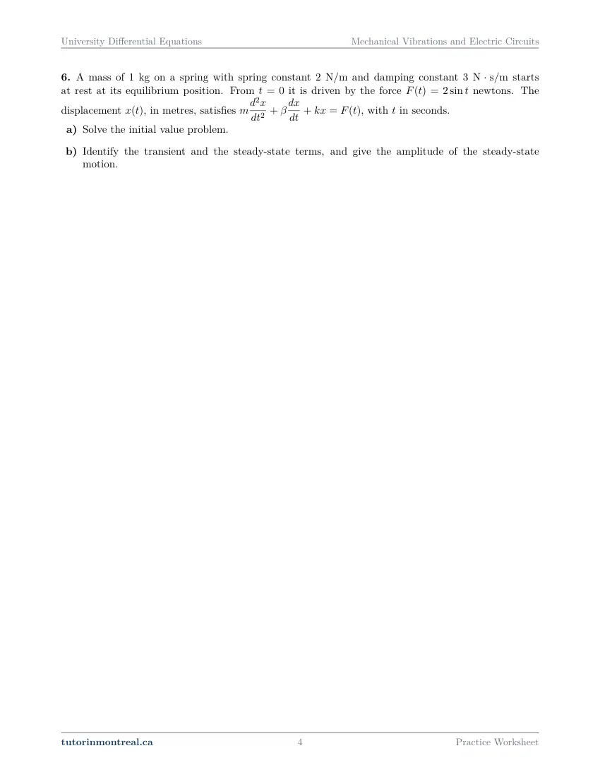
6. Q6Driven Motion with Transient and Steady-State Terms

   A mass of $1\text{kg}$ on a spring with spring constant $2\text{N}/\text{m}$ and damping constant $3\text{N}·\text{s}/\text{m}$ starts at rest at its equilibrium position. From $t=0$ it is driven by the force $F(t)=2\sin t$ newtons. The displacement $x(t)$, in metres, satisfies $m{\displaystyle \frac{d^{2}x}{d{t}^2}}+\beta {\displaystyle \frac{dx}{dt}}+kx=F(t)$, with $t$ in seconds.

   1. Solve the initial value problem.
   2. Identify the transient and the steady-state terms, and give the amplitude of the steady-state motion.
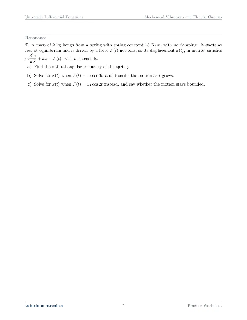
7. Q7Resonance

   A mass of $2\text{kg}$ hangs from a spring with spring constant $18\text{N}/\text{m}$, with no damping. It starts at rest at equilibrium and is driven by a force $F(t)$ newtons, so its displacement $x(t)$, in metres, satisfies $m{\displaystyle \frac{d^{2}x}{d{t}^2}}+kx=F(t)$, with $t$ in seconds.

   1. Find the natural angular frequency of the spring.
   2. Solve for $x(t)$ when $F(t)=12\cos 3t$, and describe the motion as $t$ grows.
   3. Solve for $x(t)$ when $F(t)=12\cos 2t$ instead, and say whether the motion stays bounded.
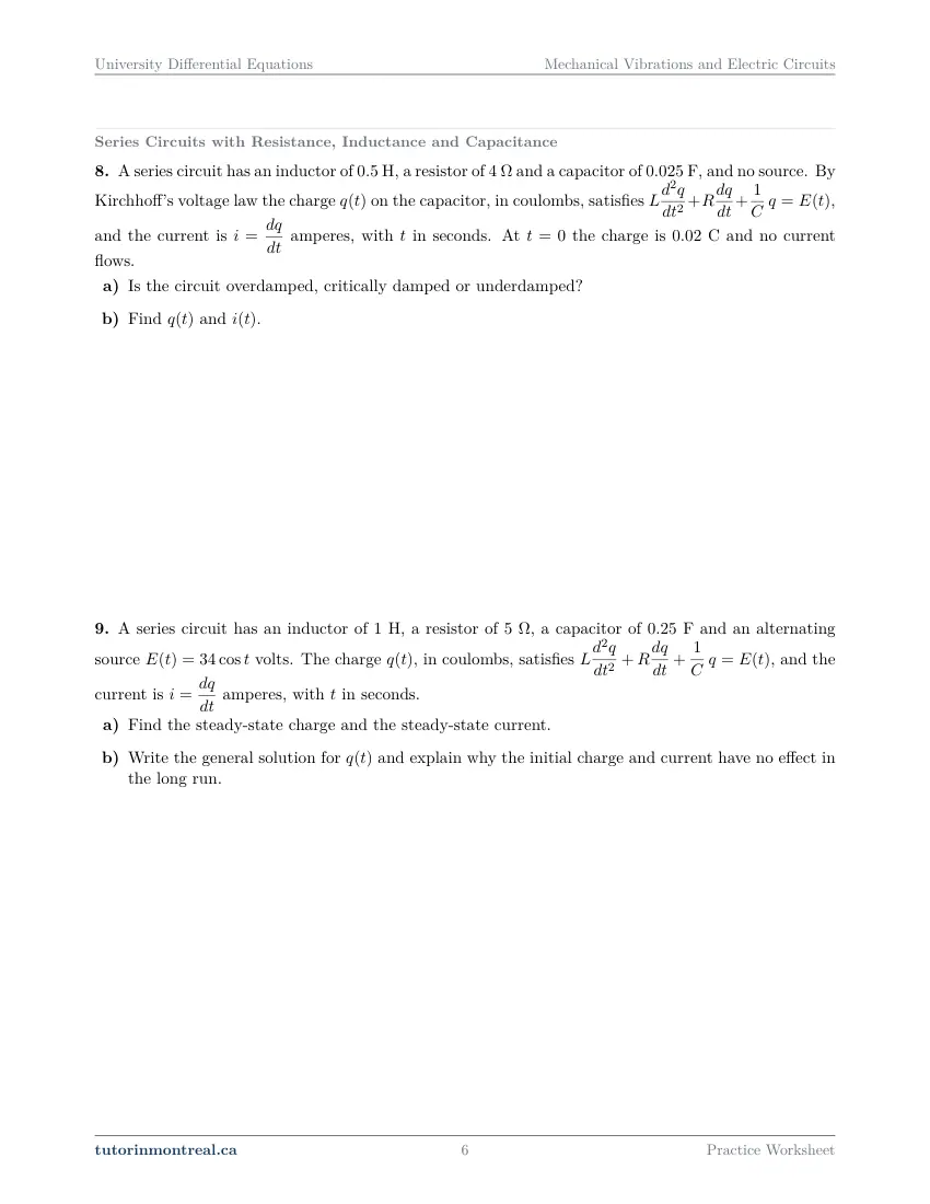
8. Q8Series Circuits with Resistance, Inductance and Capacitance

   A series circuit has an inductor of $0.5\text{H}$, a resistor of $4\Omega$ and a capacitor of $0.025\text{F}$, and no source. By Kirchhoff's voltage law the charge $q(t)$ on the capacitor, in coulombs, satisfies $L{\displaystyle \frac{d^{2}q}{d{t}^2}}+R{\displaystyle \frac{dq}{dt}}+{\displaystyle \frac{1}{C}}q=E(t)$, and the current is $i={\displaystyle \frac{dq}{dt}}$ amperes, with $t$ in seconds. At $t=0$ the charge is $0.02\text{C}$ and no current flows.

   1. Is the circuit overdamped, critically damped or underdamped?
   2. Find $q(t)$ and $i(t)$.
9. Q9Series Circuits with Resistance, Inductance and Capacitance

   A series circuit has an inductor of $1\text{H}$, a resistor of $5\Omega$, a capacitor of $0.25\text{F}$ and an alternating source $E(t)=34\cos t$ volts. The charge $q(t)$, in coulombs, satisfies $L{\displaystyle \frac{d^{2}q}{d{t}^2}}+R{\displaystyle \frac{dq}{dt}}+{\displaystyle \frac{1}{C}}q=E(t)$, and the current is $i={\displaystyle \frac{dq}{dt}}$ amperes, with $t$ in seconds.

   1. Find the steady-state charge and the steady-state current.
   2. Write the general solution for $q(t)$ and explain why the initial charge and current have no effect in the long run.
10. Q10Synthesis — drawing on several topics in this unit

    A series circuit has an inductor of $2\text{H}$, a resistor of $8\Omega$ and a capacitor of $0.1\text{F}$. A $20\text{V}$ battery is switched in at $t=0$, when the capacitor is uncharged and no current flows. The charge $q(t)$, in coulombs, satisfies $L{\displaystyle \frac{d^{2}q}{d{t}^2}}+R{\displaystyle \frac{dq}{dt}}+{\displaystyle \frac{1}{C}}q=E(t)$, and the current is $i={\displaystyle \frac{dq}{dt}}$ amperes, with $t$ in seconds.

    1. Classify the circuit as overdamped, critically damped or underdamped.
    2. Find $q(t)$ and $i(t)$.
    3. Identify the steady-state charge and the transient part.

The 6 challenge problems for this topic are a separate, paid sheet and are not reproduced here.

How to do every concept on this sheet

This is the part worksheet sites usually leave out. Below is the actual reasoning behind each group of questions — not a full solution set, the decisions that get you to one. Read it before you start, or after you get stuck.

One equation, many machines

Every question in this set is an instance of the same constant-coefficient equation. What changes from one question to the next is which terms are present and what the letters stand for. Before solving anything, write the equation with the numbers in it and say what each coefficient is — a mass, a damping constant, a spring constant; or an inductance, a resistance, a reciprocal capacitance.

Free undamped motion and the amplitude-phase form

With no damping and no force, the characteristic equation has purely imaginary roots, and the solution is a combination of cos(ωt) and sin(ωt) with ω = √(k/m), the natural angular frequency. Q1 asks for that solution from two initial conditions, and then for the same function rewritten as a single shifted cosine, A cos(ωt − δ). That form is what makes the physical questions answerable at a glance: A is the amplitude, 2π/ω is the period, and the times at which the mass passes through equilibrium are where the cosine is zero.

Q1(c) asks two things the amplitude-phase form answers without further calculus. The first passage through equilibrium is the first t > 0 where ωt − δ reaches an odd multiple of π/2 — pick the smallest one that gives a positive time. The greatest speed is the largest value of |x′|, and differentiating A cos(ωt − δ) shows directly what that is in terms of A and ω.

Q2 starts one step earlier: the spring constant is not given, only how far the mass stretches the spring at rest. Hanging at rest, the mass feels two equal and opposite forces, its weight and the pull of the spring, which makes k times the static stretch equal to mg — that is the whole of part (a) before ω. Part (b) is Q1 again with the sign convention doing the work: "above" and "upward" are both negative here. Part (c) asks for the frequency in oscillations per second, which is not ω: ω counts radians per second, so divide by 2π.

Damping: which of the three cases?

A dashpot adds the term β x′, and the characteristic equation m r² + β r + k = 0 now has a discriminant that can be positive, zero or negative. That sign is the whole classification, and Q3 asks for nothing else: three values of β on the same mass and spring, a verdict for each, and the general solution each verdict produces.

Q4 takes one underdamped system all the way. Part (a) is the initial value problem; mind that the derivative of e^(−λt) cos μt has two terms, so the initial velocity involves both constants. Part (b) is Q1's amplitude-phase conversion applied to the bracket only — the exponential factor stays outside — and the quasi-period is 2π/μ, the time between successive peaks of the oscillation. It is not a true period, because the motion never repeats exactly.

Driven motion: the transient and the steady state

Add a periodic force and the equation becomes nonhomogeneous. The general solution is the complementary solution plus a particular one, and with damping present those two pieces have names. The complementary part carries a decaying exponential in every term, so it fades: that is the transient. The particular part oscillates at the driving frequency for as long as the force acts: that is the steady state.

Q5 walks through it in the order the method runs. Part (a) gives the trial form A cos t + B sin t, so substitute it, collect the cosine terms and the sine terms separately, and solve the two linear equations for A and B. Part (b) adds the complementary solution — find the characteristic roots first, since their real part is what makes the transient label earned rather than assumed. Part (c) is the amplitude of the steady state: the particular solution is a combination of a cosine and a sine at one frequency, so its amplitude is √(A² + B²), exactly as in Q1.

Q6(b) then asks you to sort the terms of your answer. The test is the one from Q5: a term with a decaying exponential factor is transient; a term that oscillates with the forcing frequency and no decay is steady state. Note that the forcing here is a sine rather than a cosine; the trial solution still needs both a cosine and a sine.

Resonance: when the force keeps time with the spring

Q7 removes the damping and compares two driving forces with different frequencies. Part (a) is the number everything turns on: the natural angular frequency √(k/m). Parts (b) and (c) are decided by comparing each forcing frequency with it.

The series circuit is the same equation

Kirchhoff's voltage law gives L q″ + R q′ + (1/C) q = E(t) for the charge on the capacitor, and every tool above carries over under the dictionary L ↔ m, R ↔ β, 1/C ↔ k, E(t) ↔ F(t). The current is i = q′, so once q is known, the current is one derivative away.

Q8(b) is an initial value problem like Q4's: the initial charge gives q(0), and "no current flows" is the statement q′(0) = 0. Differentiate your charge to give the current, and check that it vanishes at t = 0.

Q9 drives the circuit with an alternating source, and part (a) asks only for the steady state — the particular solution, found by undetermined coefficients exactly as in Q5, with the steady- state current as its derivative. Part (b) asks for the general solution and an explanation, and the explanation is the one Q5 set up: look at the characteristic roots, say what their real parts do to the complementary terms as t grows, and connect that to where the initial charge and current enter the solution.

The synthesis question

Q10 switches a battery into an uncharged circuit and asks for the whole story in three steps. Part (a) is Q8(a) with new numbers. Part (b) needs a particular solution for a constant source, and the trial solution for a constant right-hand side is a constant; substitute it and the derivative terms vanish. Then add the complementary solution in the form part (a)'s verdict dictates, and impose q(0) = 0 and q′(0) = 0 on the sum — Q6's order, not the complementary part alone. Part (c) uses Q5's and Q6's split: name the term that settles to a fixed value and the terms that die away, and say what the current does in the long run.

Preview all 7 pages

Click any page to open the full PDF.

Getting the most out of it

Translate the words into signed numbers first

Before solving, write the equation with its coefficients and the two initial conditions as numbers with signs. "Below", "above", "upward", "at rest", "no current" and "uncharged" are all initial conditions in disguise, and the convention for the positive direction is in the question.

Classify before you solve

Compute the discriminant of the characteristic equation and write the damping case in words. It takes one line, it tells you which form the solution will take, and it is the part of the question most often left unjustified.

Keep ω, the frequency and the period apart

Angular frequency is in radians per second, frequency in oscillations per second, and the period in seconds per oscillation. Write the unit beside each number; it catches a missing 2π at once.

Check the long-run behaviour against the physics

With damping, the transient must decay; with a constant source, the charge must level off; with no damping and matching frequencies, something has to grow. If your formula disagrees with the physical picture, look for a sign error in the characteristic roots or a trial solution that should have been multiplied by t.

Common questions