University Differential Equations — The Laplace Transform Worksheet
The chapter that turns a differential equation into algebra. Transform both sides, and derivatives become powers of s with the initial conditions already built in; solve for Y(s) by rearranging; then transform back. The set drills each link in that chain — the transform computed from its definition and read off a table, the inverse transform by partial fractions, the two translation theorems that handle a factor eᵃᵗ and a delayed switch, the unit step that writes a piecewise forcing term as one formula, the formula for a periodic input, the convolution theorem that turns a product of transforms into an integral, and the Dirac delta that models a sudden blow. It ends with initial value problems whose right-hand sides the earlier methods of this course could not handle. Have a look on this page, then print the free PDF when you want to write on it.
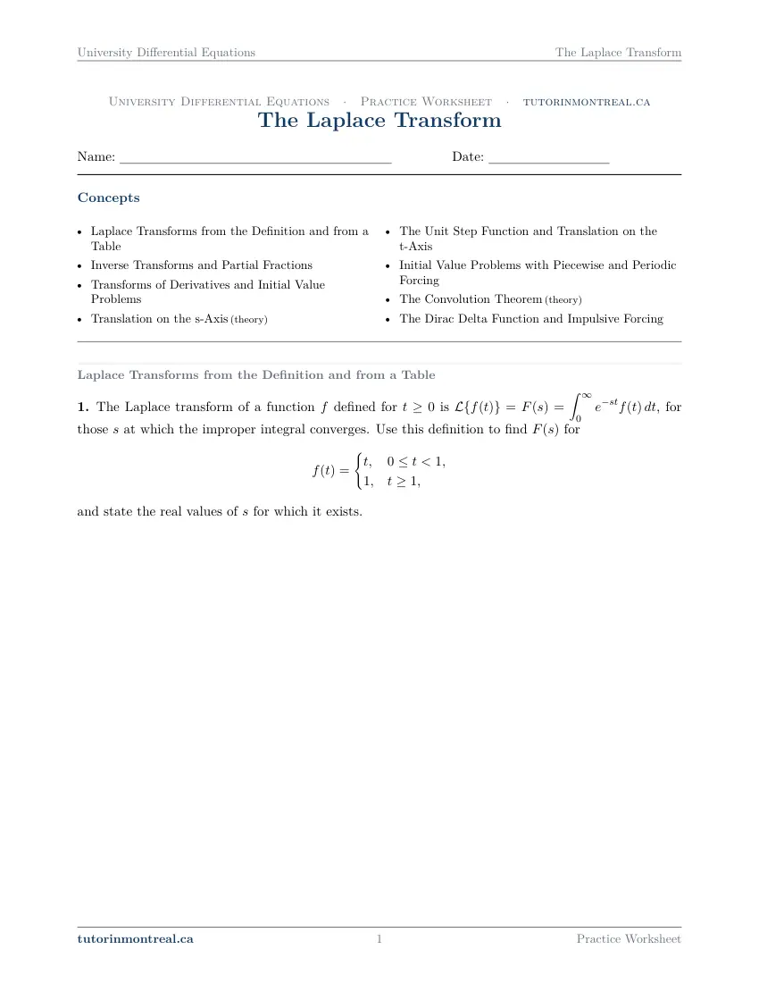
Practice worksheet — free PDF
No email, no account, no watermark. Teachers: photocopy it for your classes freely. Worked solutions and 10 harder problems come with the University Differential Equations bundle.
All 15 questions
Each question targets one named concept from the sheet. Read them here, or print the PDF — it has working space under each one.
-
Q1Laplace Transforms from the Definition and from a Table
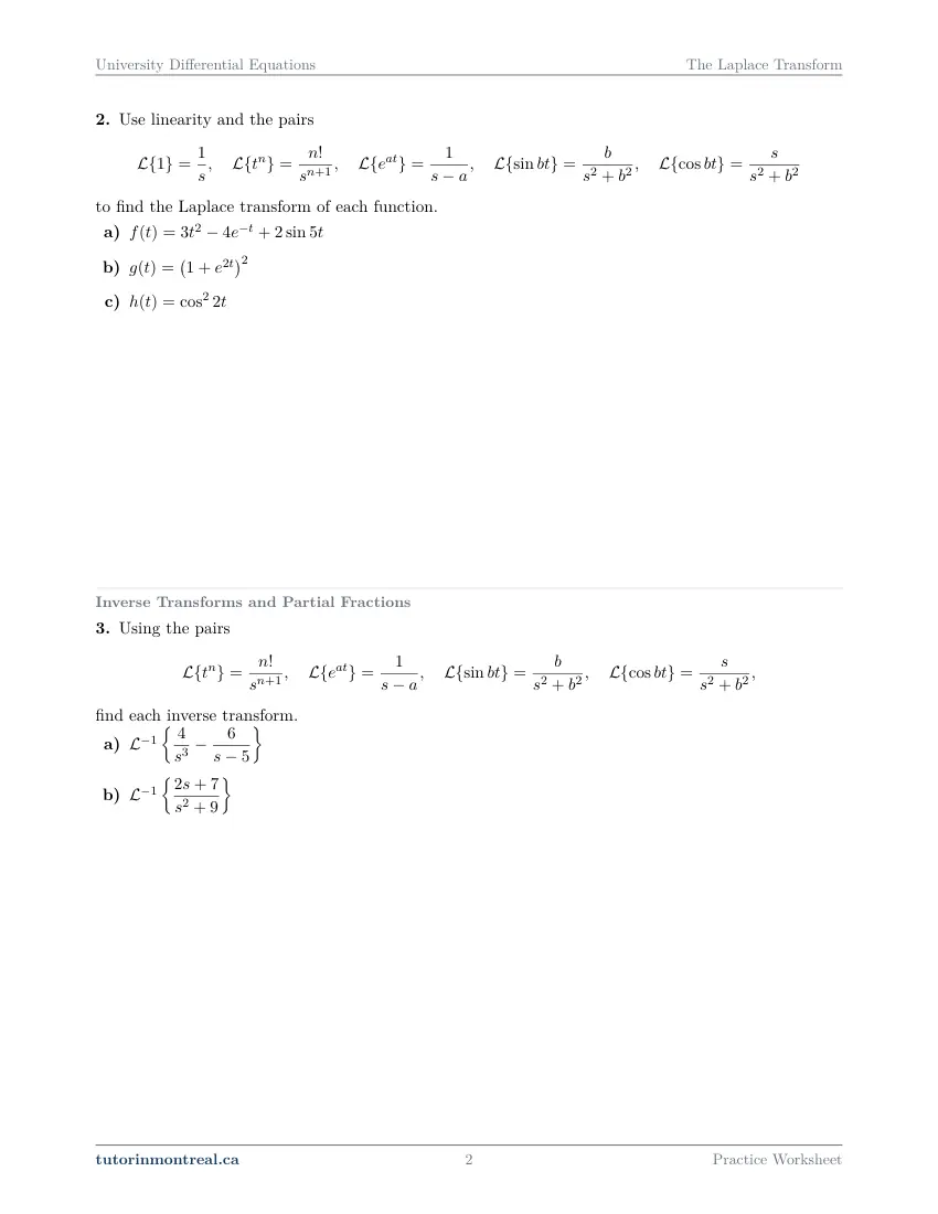
The Laplace transform of a function defined for is , for those at which the improper integral converges. Use this definition to find for and state the real values of for which it exists.
-
Q2Laplace Transforms from the Definition and from a Table
Use linearity and the pairs to find the Laplace transform of each function.
-
Q3Inverse Transforms and Partial Fractions
Using the pairs find each inverse transform.
-
Q4Inverse Transforms and Partial Fractions
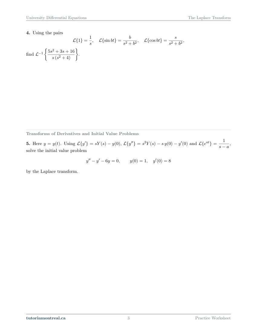
Using the pairs find .
-
Q5Transforms of Derivatives and Initial Value Problems
Here . Using , and , solve the initial value problem by the Laplace transform.
-
Q6Transforms of Derivatives and Initial Value Problems
Here . Using and solve by the Laplace transform.
-
Q7Translation on the s-Axis
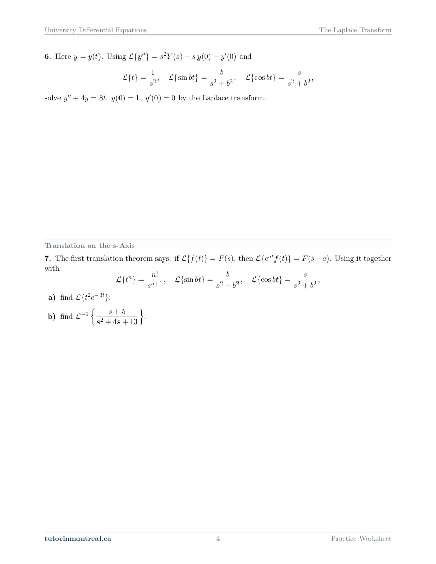
The first translation theorem says: if , then . Using it together with
- find ;
- find .
-
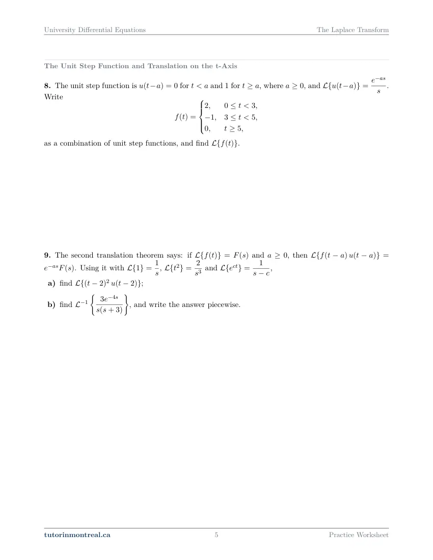
Q8The Unit Step Function and Translation on the t-Axis
The unit step function is for and for , where , and . Write as a combination of unit step functions, and find .
-
Q9The Unit Step Function and Translation on the t-Axis
The second translation theorem says: if and , then . Using it with , and ,
- find ;
- find , and write the answer piecewise.
-
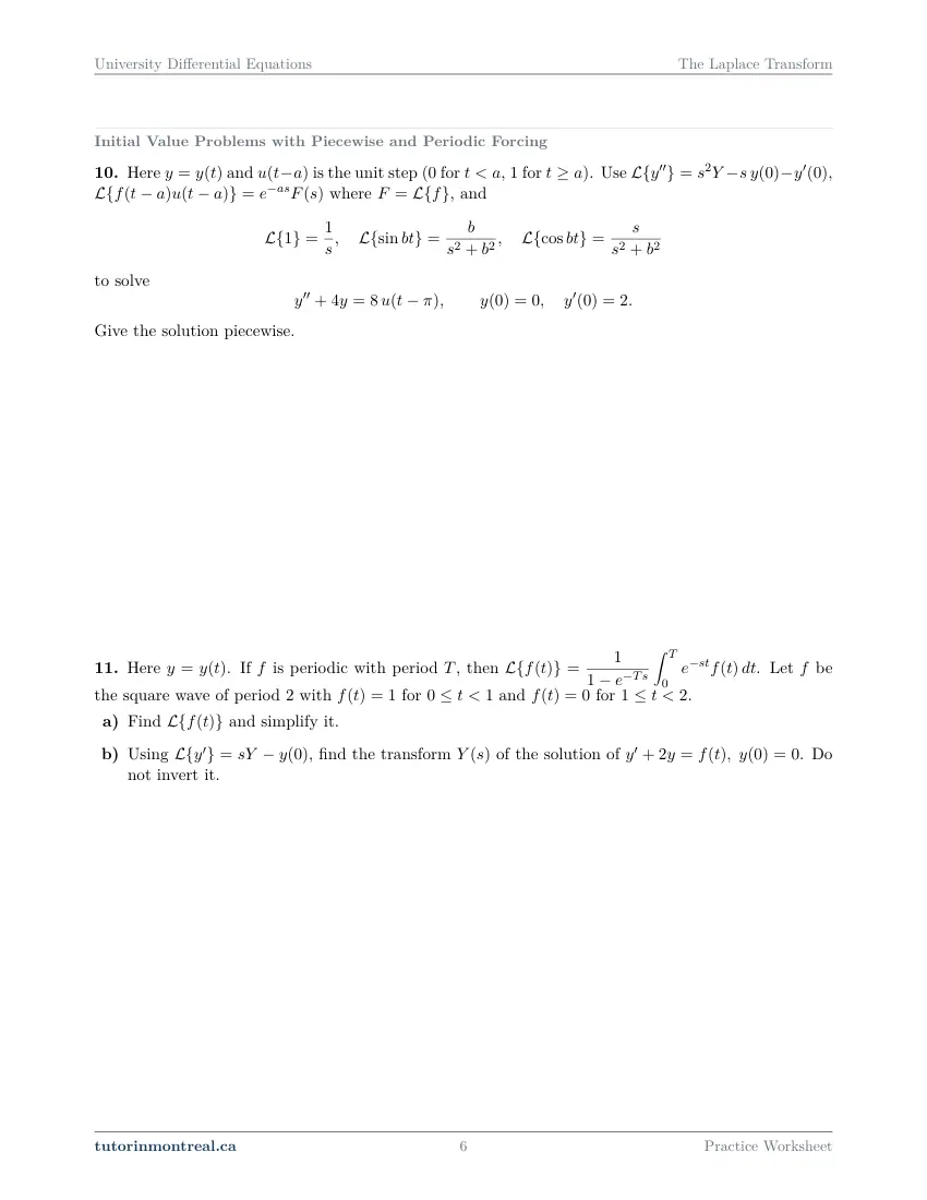
Q10Initial Value Problems with Piecewise and Periodic Forcing
Here and is the unit step ( for , for ). Use , where , and to solve Give the solution piecewise.
-
Q11Initial Value Problems with Piecewise and Periodic Forcing
Here . If is periodic with period , then . Let be the square wave of period with for and for .
- Find and simplify it.
- Using , find the transform of the solution of . Do not invert it.
-
Q12The Convolution Theorem
The convolution of and is , and the convolution theorem says .
- Compute from the definition.
- Check your answer by finding its inverse transform another way: invert by partial fractions, using , , .
-
Q13The Dirac Delta Function and Impulsive Forcing
Here , is the Dirac delta at , with , and is the unit step ( for , for ). Using , and , solve and state how the impulse changes at .
-
Q14The Dirac Delta Function and Impulsive Forcing
Here , is the Dirac delta at , with , and is the unit step. Using , , and , solve
-
Q15Synthesis — drawing on several topics in this unit
Here and is the unit step ( for , for ). Using , , , and , solve and find .
The 10 challenge problems for this topic are a separate, paid sheet and are not reproduced here.
What does this set assume? This set stands on CEGEP Calculus I and II and re-teaches none of them. Improper integrals and their convergence, integration by parts, and partial fractions — including an irreducible quadratic factor — are used without comment, because the transform is defined by an improper integral and inverted by partial fractions. From the earlier University Differential Equations sets it assumes Homogeneous Linear Equations with Constant Coefficients and Nonhomogeneous Equations and Variable Coefficients, so that you can check a Laplace answer against the characteristic equation or a trial solution, and the forcing language of Mechanical Vibrations and Electric Circuits. Tables are assumed: each question prints the pairs it needs, and a question may expect you to read one off rather than derive it. Transfer functions are not in this course, systems are solved by the eigenvalue method rather than by the transform, and Fourier series and partial differential equations are out of the course altogether.
Which course is this for? In the public course calendars of Montreal universities, this material is part of the courses numbered MATH 263, MATH 315 and MAT265. Each course orders and weights the topics its own way, so check your own outline for what your exam covers. Which sets match your course.
How to do every concept on this sheet
This is the part worksheet sites usually leave out. Below is the actual reasoning behind each group of questions — not a full solution set, the decisions that get you to one. Read it before you start, or after you get stuck.
The transform from its definition
The Laplace transform of f is an improper integral, ℒ{f} = F(s) = ∫₀^∞ e^(−st) f(t) dt, and it exists only for the values of s that make that integral converge. Q1 asks for it from the definition, for a function given in two pieces, and asks for the values of s as well as the formula. Both halves are marked.
split the integral where f changes formula → integrate each piece → take the limit as the upper bound → ∞A piecewise function means a split integral. Write one integral from 0 to the break point with the first formula and one from the break point to infinity with the second. The finite piece with a factor of t in it needs integration by parts; the infinite piece is where the convergence question lives, because it is the one written as a limit.
Decide where it converges before you simplify. The term e^(−st) goes to zero as t → ∞ only for some values of s. Settle that on the unsimplified limit, and treat any boundary value of s on its own by substituting it into the original integral — a formula you reach by dividing by s says nothing about what happens when s is zero.
Q2 is the table and the fact that makes the table enough: the transform is linear, so a sum of constant multiples transforms term by term. Part (a) is already in that form. Parts (b) and (c) are not, and the work is to rewrite them until they are — expand the square in (b), and in (c) use a double-angle identity to replace the square of a cosine by something linear in cosines. There is no table entry for a product or a square, so a function that is not already a sum of table entries has to be made into one first.
Inverse transforms and partial fractions
Going back from F(s) to f(t) is reading the table in reverse, and almost all of the work is making F(s) look like a table entry. Q3 has two shapes. In part (a) each term already matches a pair except for its constant, and the constant is adjusted: the pair for tⁿ carries n! on top, so a different numerator means multiplying and dividing by what is missing. In part (b) the numerator has an s term and a constant term over s² + b².
Split the numerator before you look anything up. A numerator of the form (ps + q) over s² + b² is two fractions: the s part matches the cosine entry, the constant part matches the sine entry once you arrange for exactly b to sit on top. Make the constant fit the entry by multiplying and dividing — never change the denominator to fit the numerator.
Q4 needs partial fractions first. The denominator is s times an irreducible quadratic, so the decomposition has a constant over s and a linear term over the quadratic. Find the constants by clearing denominators and comparing coefficients (or substituting a convenient s), then invert each piece exactly as in Q3.
linear factor s − a → A/(s − a) irreducible quadratic → (Bs + C)/(quadratic)Transforms of derivatives and initial value problems
The reason the transform belongs in this course is one formula: the transform of y′ is sY(s) − y(0), and of y″ is s²Y(s) − s y(0) − y′(0). The initial conditions go in at the start, not at the end — there is no general solution with arbitrary constants to fit afterwards.
Solving an initial value problem by the Laplace transform
Four steps, the same every time.
- 1Transform both sides
Replace each derivative by its formula with the given initial values substituted, and transform the right-hand side from the table.
- 2Solve for Y(s)
Collect every Y term on one side and factor; what multiplies Y is the characteristic polynomial in s. Divide.
- 3Decompose
Partial fractions, one term per factor of the denominator, until every piece is a table entry.
- 4Invert and check
Transform back term by term, then check y(0) and y′(0) in your answer. Both are free marks.
Q5 is a homogeneous equation: after step 2 the only thing on the right is what the initial conditions produced, and the denominator is a quadratic in s to factor. Q6 has a forcing term, so Y(s) has two parts, one from the forcing and one from the initial conditions, and the forcing part has a repeated factor of s in the denominator as well as s² + 4.
Signs in the derivative formulas are the usual loss. Every initial value enters with a minus sign, and the y(0) in the formula for y″ is multiplied by s. Write the formula out with the numbers substituted before you move anything across the equals sign.
Translation on the s-axis
Multiplying a function by eᵃᵗ shifts its transform: F(s) becomes F(s − a). Q7 uses the theorem in both directions. Part (a) is forwards — find the transform of the power alone, then replace every s by s − a. Part (b) is backwards, and needs a recognisable shift first.
complete the square in the denominator → (s − a)² + b² → rewrite the numerator in terms of s − aThe numerator has to be shifted too. Once the denominator reads (s − a)² + b², the numerator must be written as a multiple of (s − a) plus a constant, because those are the two pieces the shifted cosine and sine entries expect. Then adjust the constant to b, exactly as in Q3, and put the factor eᵃᵗ on both pieces.
Read the sign of a off the square. A denominator of (s + 2)² + … is (s − a)² with a negative a, so the exponential decays. Getting that sign backwards is the most common error with this theorem.
The unit step and translation on the t-axis
The unit step u(t − a) is 0 before a and 1 from a on. It is a switch, and a piecewise function is a sum of switches. Q8 asks you to write a three-piece function that way and then transform it.
Build it jump by jump. Start with the value on the first piece. At each break point add a step whose coefficient is the change in value there — the new value minus the old one, with its sign. Check the result by evaluating it on each interval; it must give back the function you were given. Only then transform, one step at a time, using the entry for u(t − a).
The second translation theorem says that delaying a function by a — writing f(t − a) u(t − a) — multiplies its transform by e^(−as). Q9(a) is that statement used forwards: identify what f is once the delay is taken out. Q9(b) is it used backwards, and the exponential is a label, not part of the algebra.
Inverting a transform that carries e^(−as)
Set the exponential aside, then put the delay back.
- 1Remove the exponential
Write the transform as e^(−as) times F(s). Everything that follows is about F alone.
- 2Invert F
Partial fractions if needed; this gives f(t).
- 3Delay it
Replace every t by t − a and multiply by u(t − a). Every t, including the one inside each exponential.
- 4Write it piecewise
Q9(b) asks for this: one formula before a, where the step is 0, and one from a on.
Piecewise and periodic forcing
Q10 is the reason the step function is in this chapter: a forcing term that switches on at t = π, which a trial solution could only handle interval by interval. Transformed, it is one equation. Y(s) splits into the part from the initial conditions and the part from the switched forcing; the second carries e^(−πs), so invert it with the tree above — partial fractions on the rest, then delay.
Simplify the shifted trigonometric terms. After the delay you will have sines and cosines of 2(t − π). Before writing the piecewise answer, use the period of those functions to rewrite them in terms of 2t; the question asks for the solution piecewise, and each piece should be as simple as it can be.
Q11 gives the formula for a periodic function: the integral over one period, divided by 1 − e^(−Ts). Part (a) needs only the part of the period where the square wave is non-zero, since the rest contributes nothing to the integral; then look for a factorisation of the denominator that cancels with the numerator. Part (b) transforms a first-order equation with that forcing and stops at Y(s) — the question says not to invert, so the answer is a transform.
The convolution theorem
The transform of a product is not the product of the transforms. What does have a product of transforms as its transform is the convolution (f ∗ g)(t) = ∫₀ᵗ f(τ) g(t − τ) dτ. Q12 computes one convolution two ways, and the two answers must agree.
τ is the variable; t is a constant inside the integral. In part (a), substitute τ for the first function and t − τ for the second, then integrate with respect to τ. Any factor that depends only on t comes out in front of the integral. What is left is an integration by parts. In part (b), the denominator has a repeated factor of s, so the decomposition needs a term over s and a term over s² as well as one over s − 1.
The Dirac delta and impulsive forcing
δ(t − a) models a blow delivered all at once at time a: its transform is e^(−as), which is what you get from the step-function formula if you imagine a very tall, very short pulse of total area 1. In an equation it behaves like any other right-hand side with an exponential label — transform, solve for Y, invert with the delay.
Q13 is first order. Its solution is one formula before t = 1 and another after, joined by a step, and the question asks what the impulse does to y at that moment.
Read the effect off your solution. Compute the limit of y as t approaches 1 from the left and the value at 1 from the formula on the right, and compare them. The answer to "how does the impulse change y" is that comparison, stated in words: whether y is continuous at t = 1, and if not, by how much and in which direction it moves.
Q14 is second order, with a damped left-hand side, so the denominator of Y(s) is a quadratic you complete the square in — Q7's technique. The table pairs printed with the question are exactly the shifted cosine and sine you will need. The impulse term carries e^(−2s), so it is inverted with the delay; the initial-condition terms are not.
Check the delayed term at the moment it switches on. A delayed term written as f(t − a) u(t − a) is zero just before a; evaluate your f at t − a = 0 to see what it contributes just after. Comparing the two sides of t = 2 for y and for y′ is a quick test that the delay was applied to every t.
The synthesis question
Q15 puts the chapter together: a second-order equation with a switched constant forcing and non-zero initial slope. It is Q5's four steps with Q10's delay. The part from the switched forcing has three factors in its denominator — one from the step, two from the characteristic polynomial — so its partial fractions have three terms before you delay them.
The limit is read from the form of the answer, not computed from scratch. Once t is past the switch, write y as a sum of terms. Any term that is a decaying exponential tends to zero; a constant stays. Decide which of your terms are which from the sign in each exponent, and the limit is what remains.
Preview all 9 pages
Click any page to open the full PDF.
Getting the most out of it
Keep the table in front of you, and use only its entries
Every question prints the pairs it expects. Work from those. The whole skill of this chapter is rewriting an expression until each piece matches an entry exactly — including the constant on top — and adjusting by multiplying and dividing, never by changing a denominator.
Write the initial values in at step one
Substitute y(0) and y′(0) into the derivative formulas as soon as you transform. A Laplace solution has no arbitrary constants; if you find yourself fitting one at the end, something went wrong earlier.
Set exponentials aside before partial fractions
A factor e^(−as) is never part of a partial-fraction decomposition. Pull it out, decompose and invert what is left, then apply the delay to the whole of the result. Mark which terms carry a delay before you start, so none is inverted as if it did not.
Check the answer in the equation you started from
Evaluate your solution at t = 0 to check the initial values, and on each interval of a piecewise answer check that it satisfies the equation. For Q5 and Q6, the characteristic-equation methods from the earlier sets give an independent second answer.
Want the solutions, or something more challenging?
The worksheet, the questions above and every explanation on this page stay free permanently. Three more PDFs exist for this topic — the worked answer key, a harder problem set, and the answer key to that. They come with the University Differential Equations Solutions Bundle, beside the unit notes and the unit test, which is what keeps the rest of the series free.
What else exists for The Laplace Transform
Three PDFs · 18 pages · all three are in the bundle below.
- Answer key — 4 pages. All 15 questions worked step by step, including the restrictions and the justifications. Not a list of final answers.
- Challenge problems — 10 pages, 10 problems. A separate sheet at exam-plus difficulty covering the same 8 concepts. Harder than anything on the free sheet.
- Challenge answer key — 4 pages. Every challenge problem worked to the same standard, with the checks shown.
- PDF, letter size, print-ready.
The one thing that's for sale
Every University Differential Equations topic — the complete Solutions Bundle
One download, one payment, the whole program. For all 9 University Differential Equations units: the worksheet, the reference notes, the challenge set, the unit test and every answer key — including this one.
- Worked solutions, not answer lists — every step written out
- Covers the whole year's program at this level
- Less than the price of one hour of tutoring — for the entire year's solutions
Taking Secondary 1 Math as well? The Secondary 1 Math bundle covers all 15 of its units — 106 PDFs, 474 pages — on the same terms.
Taking Secondary 2 Math as well? The Secondary 2 Math bundle covers all 14 of its units — 98 PDFs, 449 pages — on the same terms.
Taking Secondary 3 Math as well? The Secondary 3 Math bundle covers all 11 of its units — 77 PDFs, 367 pages — on the same terms.
Taking Secondary 4 Math as well? The Secondary 4 Math bundle covers all 17 of its units — 122 PDFs, 466 pages — on the same terms.
Taking Secondary 5 Math as well? The Secondary 5 Math bundle covers all 21 of its units — 147 PDFs, 589 pages — on the same terms.
Taking CEGEP Calculus I as well? The CEGEP Calculus I bundle covers all 9 of its units — 72 PDFs, 371 pages — on the same terms.
Taking CEGEP Calculus II as well? The CEGEP Calculus II bundle covers all 8 of its units — 64 PDFs, 335 pages — on the same terms.
Taking CEGEP Linear Algebra as well? The CEGEP Linear Algebra bundle covers all 7 of its units — 56 PDFs, 298 pages — on the same terms.
Taking University Calculus III as well? The University Calculus III bundle covers all 9 of its units — 72 PDFs, 516 pages — on the same terms.
Taking University Linear Algebra as well? The University Linear Algebra bundle covers all 9 of its units — 72 PDFs, 496 pages — on the same terms.
Taking University Business Math as well? The University Business Math bundle covers all 9 of its units — 36 PDFs, 190 pages — on the same terms.
Taking University Introductory Statistics as well? The University Introductory Statistics bundle covers all 9 of its units — 36 PDFs, 186 pages — on the same terms.
Taking University Discrete Math as well? The University Discrete Math bundle covers all 9 of its units — 36 PDFs, 155 pages — on the same terms.
Taking AP Calculus AB as well? The AP Calculus AB bundle covers all 8 of its units — 64 PDFs, 527 pages — on the same terms.
Common questions
Is this worksheet really free?
Yes — the questions are on this page to read, and the PDF downloads directly, no email and no account. The one paid item is optional: the complete University Differential Equations Solutions Bundle, which covers every set at this level.
Which university courses is this for?
The course codes listed on this page are taken from the public course calendars of universities that teach a first course in ordinary differential equations after CEGEP. Each course orders and weights the chapters its own way, and some reach the Laplace transform later than others or not at all, so check the outline for your own section to see where this set falls in your term.
What do I need to know before starting this set?
CEGEP Calculus I and II — improper integrals, integration by parts and partial fractions with an irreducible quadratic factor — and the earlier University Differential Equations sets on constant-coefficient equations, so that the characteristic polynomial is familiar when it reappears in s.
Why use the Laplace transform when the characteristic equation already works?
For a smooth forcing term the two methods agree, and Q5 and Q6 are there so you can check one against the other. The transform earns its place when the forcing switches on, switches off, repeats or arrives as an impulse: a trial solution would have to be fitted interval by interval, while the transform handles the whole problem as one equation.
Do I have to memorise the table?
Not for this set. Every question prints the pairs it needs, and the course assumes tables. What you do need is fluency in making an expression match an entry: splitting numerators, completing the square and adjusting constants.
What is the difference between the two translation theorems?
The first multiplies a function by eᵃᵗ and shifts its transform in s. The second delays a function by a, switching it on with u(t − a), and multiplies its transform by e^(−as). An exponential in t means the first; an exponential in s means the second.
Is the Dirac delta really a function?
Not in the ordinary sense — no function is zero everywhere but one point and still has area 1. In this course it is used through its transform, e^(−as), and through what it does to a solution: an instantaneous change at the moment of the impulse.
Are transfer functions or solving systems by Laplace transform in this set?
No. Transfer functions are not part of this course, and systems of equations are solved later by the eigenvalue method rather than by the transform.
Can teachers use this in class?
Yes. Print and photocopy it for your own classes freely — I just ask that the tutorinmontreal.ca footer stays on the page.
I'm stuck on one question. Can you help?
Yes — through one-on-one tutoring, in Montreal or online. Get in touch to arrange a session, or see the current rates.
← All 9 University Differential Equations worksheets · Secondary 1 Math series (15 sheets) → · Secondary 2 Math series (14 sheets) → · Secondary 3 Math series (11 sheets) → · Secondary 4 Math series (17 sheets) → · Secondary 5 Math series (21 sheets) → · CEGEP Calculus I series (9 sheets) → · CEGEP Calculus II series (8 sheets) → · CEGEP Linear Algebra series (7 sheets) → · University Calculus III series (9 sheets) → · University Linear Algebra series (9 sheets) → · University Business Math series (9 sheets) → · University Introductory Statistics series (9 sheets) → · University Discrete Math series (9 sheets) → · AP Calculus AB series (8 sheets) →