University Differential Equations — Nonhomogeneous Equations and Variable Coefficients Worksheet

All 10 questions

Each question targets one named concept from the sheet. Read them here, or print the PDF — it has working space under each one.

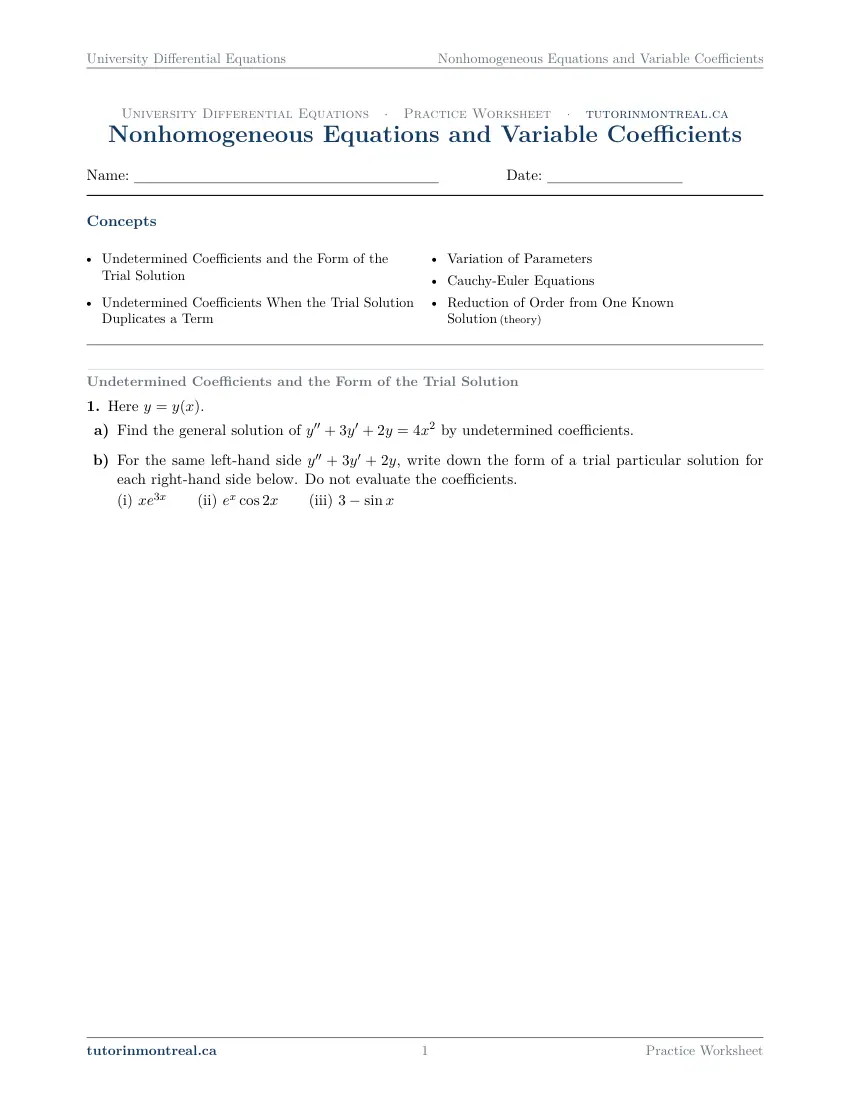
1. Q1Undetermined Coefficients and the Form of the Trial Solution

   Here $y=y(x)$.

   1. Find the general solution of $y^{″}+3y^{\prime }+2y=4x^2$ by undetermined coefficients.
   2. For the same left-hand side $y^{″}+3y^{\prime }+2y$, write down the form of a trial particular solution for each right-hand side below. Do not evaluate the coefficients.\\ (i) $x{e}^{3x}$ (ii) $e^x\cos 2x$ (iii) $3-\sin x$
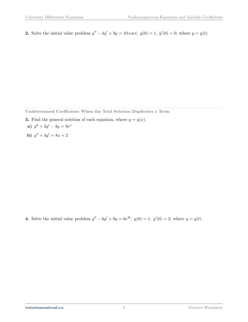
2. Q2Undetermined Coefficients and the Form of the Trial Solution

   Solve the initial value problem $y^{″}-4y^{\prime }+3y=10\cos t,y(0)=1,y^{\prime }(0)=0$, where $y=y(t)$.

3. Q3Undetermined Coefficients When the Trial Solution Duplicates a Term

   Find the general solution of each equation, where $y=y(x)$.

   1. $y^{″}+2y^{\prime }-3y=8e^x$
   2. $y^{″}+4y^{\prime }=8x+2$
4. Q4Undetermined Coefficients When the Trial Solution Duplicates a Term

   Solve the initial value problem $y^{″}-6y^{\prime }+9y=6e^{3t},y(0)=1,y^{\prime }(0)=2$, where $y=y(t)$.

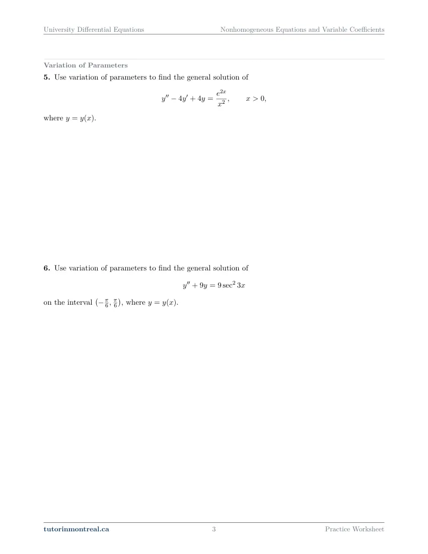
5. Q5Variation of Parameters

   Use variation of parameters to find the general solution of $$y^{″}-4y^{\prime }+4y=\frac{e^{2x}}{x^2},x>0,$$ where $y=y(x)$.

6. Q6Variation of Parameters

   Use variation of parameters to find the general solution of $$y^{″}+9y=9{\sec }^{2}3x$$ on the interval $(-\frac{\pi }{6},\frac{\pi }{6})$, where $y=y(x)$.

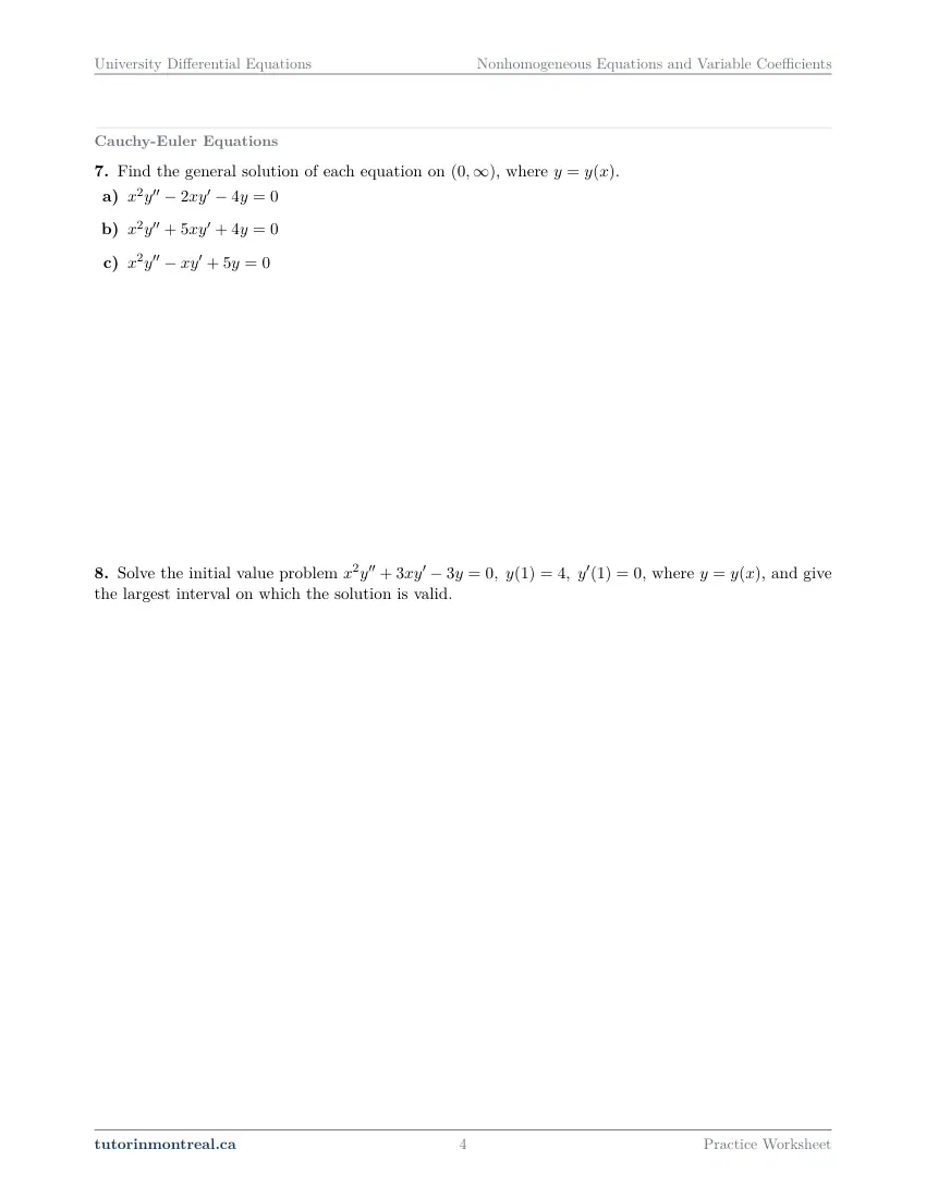
7. Q7Cauchy-Euler Equations

   Find the general solution of each equation on $(0,\infty )$, where $y=y(x)$.

   1. $x^2{y}^{″}-2x{y}^{\prime }-4y=0$
   2. $x^2{y}^{″}+5x{y}^{\prime }+4y=0$
   3. $x^2{y}^{″}-x{y}^{\prime }+5y=0$
8. Q8Cauchy-Euler Equations

   Solve the initial value problem $x^2{y}^{″}+3x{y}^{\prime }-3y=0,y(1)=4,y^{\prime }(1)=0$, where $y=y(x)$, and give the largest interval on which the solution is valid.

9. Q9Reduction of Order from One Known Solution

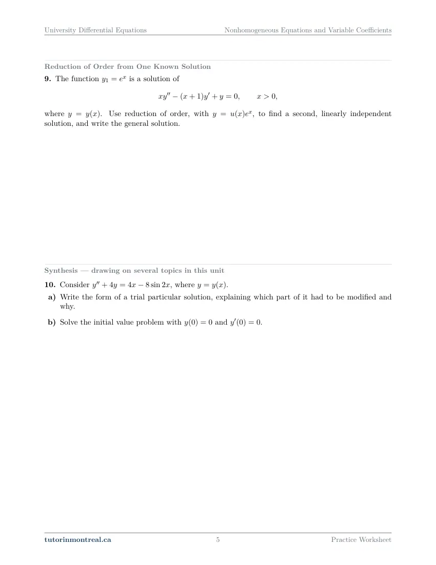
   The function $y_1=e^x$ is a solution of $$x{y}^{″}-(x+1)y^{\prime }+y=0,x>0,$$ where $y=y(x)$. Use reduction of order, with $y=u(x)e^x$, to find a second, linearly independent solution, and write the general solution.

10. Q10Synthesis — drawing on several topics in this unit

    Consider $y^{″}+4y=4x-8\sin 2x$, where $y=y(x)$.

    1. Write the form of a trial particular solution, explaining which part of it had to be modified and why.
    2. Solve the initial value problem with $y(0)=0$ and $y^{\prime }(0)=0$.

The 7 challenge problems for this topic are a separate, paid sheet and are not reproduced here.

How to do every concept on this sheet

This is the part worksheet sites usually leave out. Below is the actual reasoning behind each group of questions — not a full solution set, the decisions that get you to one. Read it before you start, or after you get stuck.

The structure every question here shares

A linear nonhomogeneous equation has a general solution with two pieces: the complementary solution y_c, which is the general solution of the same equation with the right-hand side replaced by zero, and one particular solution y_p of the equation as given. Everything in the first three sheets is a way of finding y_p; y_c always comes first, from the characteristic equation of the previous set.

Undetermined coefficients: the form of the trial solution

The method works because differentiating a polynomial, an exponential, a sine or a cosine returns more of the same family. So the guess for y_p is the most general member of the family the right-hand side belongs to, with unknown coefficients, and substituting it into the equation turns the problem into matching coefficients.

Q1(a) has a polynomial right-hand side, and the whole question turns on step 1: the forcing term is a single power of x, the guess is not. Q1(b) is the same decision three times with no arithmetic at all — for each of (i), (ii) and (iii), name the family, write the general member with letters for the coefficients, and stop. Part (iii) is a sum, so it takes step 5.

Q2 is a full initial value problem with a cosine on the right. By step 3 the guess needs a sine as well as a cosine: substitute, collect the cosine terms and the sine terms, and you get two equations in the two unknown coefficients. Then assemble y and apply the two conditions.

When the trial solution duplicates a term

If a term of your guess already solves the homogeneous equation, substituting it into the left side gives zero, and no choice of coefficient can make it equal the forcing term. The fix is the modification rule.

Q3 gives two equations and no hint about which, if either, needs the rule. In each part, find the roots of the characteristic equation, write y_c, write the unmodified guess from the forcing term, and compare term by term. In part (b), remember that a constant is a polynomial term too: ask whether a constant solves the homogeneous equation before you decide the degree of your guess.

Q4 is an initial value problem with an exponential on the right. Before choosing the guess, find the roots of the characteristic equation and count how many times the exponential's rate appears among them — that count is the power of x the guess needs, and it may be zero, one or two. Then substitute, which is heavier than usual whenever the guess carries a power of x, because the product rule is applied twice, and fit the conditions.

Variation of parameters

Undetermined coefficients needs a forcing term from a family that closes under differentiation. A quotient like the one in Q5, or a power of a secant like the one in Q6, is not in any such family, and no finite guess works. Variation of parameters replaces the constants of y_c by functions and finds them.

In Q5, start by deciding which of the three root cases the characteristic equation falls into; that fixes y₁ and y₂, and with them the Wronskian. Then write each u′ out in full and simplify before integrating — look for a factor that the forcing term and the homogeneous solutions have in common, because cancelling it first is what makes the integrals routine. The restriction x > 0 matters as soon as a logarithm appears.

Q6 pairs a trigonometric forcing term with a stated interval. Again the root case comes first. When y₁ and y₂ are trigonometric, their Wronskian simplifies through the Pythagorean identity, and the integrals that follow lean on the derivatives of secant and tangent and on standard trigonometric antiderivatives, all CEGEP Calculus II material. Use the interval in the statement: it tells you where the secant is defined and what sign it has, and so how to simplify any absolute value that an antiderivative produces.

Cauchy-Euler equations

In x²y″ + axy′ + by = 0 each derivative is multiplied by the matching power of x, so a power of x keeps its shape under the whole left-hand side. The trial solution is y = x^m, and substituting it gives a quadratic in m — the indicial equation — whose roots play the part the characteristic roots played for constant coefficients.

Q7 gives three equations, and the point of putting them side by side is that you decide the case for each from the discriminant of its indicial equation — not by eye from the original equation. Build the indicial equation from a and b carefully in every part; the coefficient of y′ has a sign that changes from part to part.

Q8 is a Cauchy-Euler initial value problem with its conditions at x = 1, which is the convenient point because every power of 1 is 1 and ln 1 = 0. The second request is new: give the largest interval on which the solution is valid. Read that off the equation, not the solution — divide by the leading coefficient to reach standard form, see where the coefficients stop being continuous, and take the interval containing the initial point.

Reduction of order from one known solution

When the coefficients are neither constant nor Cauchy-Euler, there may be no guess that works, but one known solution y₁ is enough to find a second. Q9 supplies y₁ and tells you to substitute y = u(x)y₁.

The synthesis question

Q10 puts the two undetermined-coefficients sheets on one equation. Its forcing term is a sum of a polynomial and a trigonometric term, so step 5 applies: write a guess for each piece. Part (a) then asks you to decide which of those pieces duplicates a term of y_c and to say why in words — the answer is a sentence comparing the trial terms with the complementary solution, exactly the check Q1(b) and Q3 practise. Part (b) is Q2 and Q4 together: find the coefficients piece by piece, assemble the whole solution, and only then apply the two zero conditions.

Preview all 6 pages

Click any page to open the full PDF.

Getting the most out of it

Write y_c before you write any guess

Every method in this set starts from the complementary solution — undetermined coefficients to check for duplication, variation of parameters for y₁ and y₂, the initial value problems for the full solution. Solve the homogeneous equation first, on its own line, every time.

Choose the method from the forcing term

Polynomials, exponentials, sines, cosines and their products: undetermined coefficients, which is usually faster. Anything else — a quotient, a secant, a logarithm — or variable coefficients: variation of parameters. Make the choice before you start and write it down; switching halfway wastes the most time.

Say out loud what family each term belongs to

Before writing a trial solution, name the family of each forcing term ("degree-two polynomial", "exponential times cosine") and the full general member it calls for. Q1(b) is exactly this drill; repeat it on any equation you meet until the guess comes with its missing terms already in.

Check a particular solution by substituting it

Once you have y_p, put it back into the left-hand side. It must return the forcing term exactly. This catches a wrong coefficient, a lost sign in variation of parameters and a guess that needed another factor of x, and it takes less time than re-reading your algebra.

Common questions