University Differential Equations — Systems of Linear Differential Equations Worksheet

All 11 questions

Each question targets one named concept from the sheet. Read them here, or print the PDF — it has working space under each one.

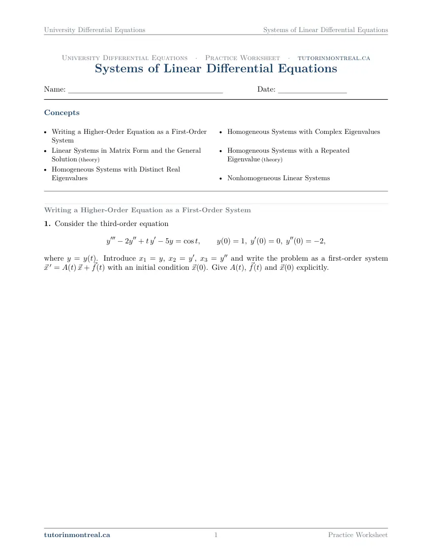
1. Q1Writing a Higher-Order Equation as a First-Order System

   Consider the third-order equation $$y^{‴}-2y^{″}+t{y}^{\prime }-5y=\cos t,y(0)=1,y^{\prime }(0)=0,y^{″}(0)=-2,$$ where $y=y(t)$. Introduce $x_1=y$, $x_2=y^{\prime }$, $x_3=y^{″}$ and write the problem as a first-order system $\overrightarrow{x}{}^{\prime }=A(t)\overrightarrow{x}+\overrightarrow{f}(t)$ with an initial condition $\overrightarrow{x}(0)$. Give $A(t)$, $\overrightarrow{f}(t)$ and $\overrightarrow{x}(0)$ explicitly.

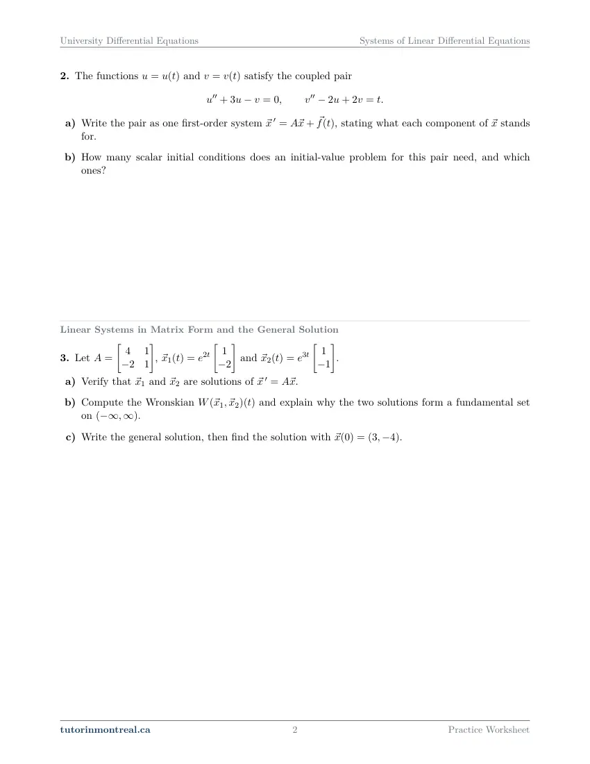
2. Q2Writing a Higher-Order Equation as a First-Order System

   The functions $u=u(t)$ and $v=v(t)$ satisfy the coupled pair $$u^{″}+3u-v=0,v^{″}-2u+2v=t.$$

   1. Write the pair as one first-order system $\overrightarrow{x}{}^{\prime }=A\overrightarrow{x}+\overrightarrow{f}(t)$, stating what each component of $\overrightarrow{x}$ stands for.
   2. How many scalar initial conditions does an initial-value problem for this pair need, and which ones?
3. Q3Linear Systems in Matrix Form and the General Solution

   Let $A=\left[\begin{array}{cc}4& 1\\ -2& 1\end{array}\right]$, ${\overrightarrow{x}}_1(t)=e^{2t}\left[\begin{array}{c}1\\ -2\end{array}\right]$ and ${\overrightarrow{x}}_2(t)=e^{3t}\left[\begin{array}{c}1\\ -1\end{array}\right]$.

   1. Verify that ${\overrightarrow{x}}_1$ and ${\overrightarrow{x}}_2$ are solutions of $\overrightarrow{x}{}^{\prime }=A\overrightarrow{x}$.
   2. Compute the Wronskian $W({\overrightarrow{x}}_1,{\overrightarrow{x}}_2)(t)$ and explain why the two solutions form a fundamental set on $(-\infty ,\infty )$.
   3. Write the general solution, then find the solution with $\overrightarrow{x}(0)=(3,-4)$.
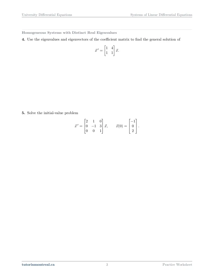
4. Q4Homogeneous Systems with Distinct Real Eigenvalues

   Use the eigenvalues and eigenvectors of the coefficient matrix to find the general solution of $$\overrightarrow{x}{}^{\prime }=\left[\begin{array}{cc}1& 4\\ 1& 1\end{array}\right]\overrightarrow{x}.$$

5. Q5Homogeneous Systems with Distinct Real Eigenvalues

   Solve the initial-value problem $$\overrightarrow{x}{}^{\prime }=\left[\begin{array}{ccc}2& 1& 0\\ 0& -1& 3\\ 0& 0& 1\end{array}\right]\overrightarrow{x},\overrightarrow{x}(0)=\left[\begin{array}{c}-1\\ 0\\ 2\end{array}\right].$$

6. Q6Homogeneous Systems with Complex Eigenvalues

   Find the general real-valued solution of $$\overrightarrow{x}{}^{\prime }=\left[\begin{array}{cc}1& -5\\ 1& -3\end{array}\right]\overrightarrow{x}.$$

7. Q7Homogeneous Systems with Complex Eigenvalues

   Solve the initial-value problem $$\overrightarrow{x}{}^{\prime }=\left[\begin{array}{cc}3& -2\\ 4& -1\end{array}\right]\overrightarrow{x},\overrightarrow{x}(0)=\left[\begin{array}{c}2\\ 3\end{array}\right].$$

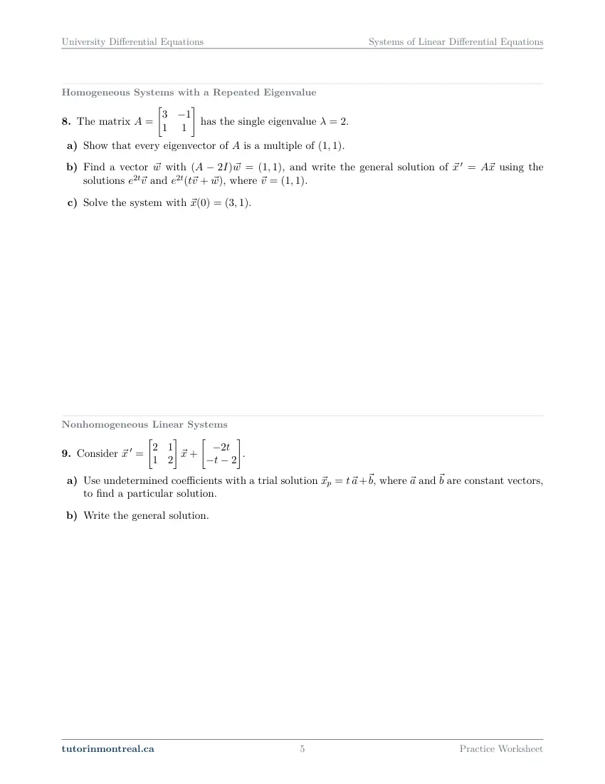
8. Q8Homogeneous Systems with a Repeated Eigenvalue

   The matrix $A=\left[\begin{array}{cc}3& -1\\ 1& 1\end{array}\right]$ has the single eigenvalue $\lambda =2$.

   1. Show that every eigenvector of $A$ is a multiple of $(1,1)$.
   2. Find a vector $\overrightarrow{w}$ with $(A-2I)\overrightarrow{w}=(1,1)$, and write the general solution of $\overrightarrow{x}{}^{\prime }=A\overrightarrow{x}$ using the solutions $e^{2t}\overrightarrow{v}$ and $e^{2t}(t\overrightarrow{v}+\overrightarrow{w})$, where $\overrightarrow{v}=(1,1)$.
   3. Solve the system with $\overrightarrow{x}(0)=(3,1)$.
9. Q9Nonhomogeneous Linear Systems

   Consider $\overrightarrow{x}{}^{\prime }=\left[\begin{array}{cc}2& 1\\ 1& 2\end{array}\right]\overrightarrow{x}+\left[\begin{array}{c}-2t\\ -t-2\end{array}\right]$.

   1. Use undetermined coefficients with a trial solution ${\overrightarrow{x}}_p=t\overrightarrow{a}+\overrightarrow{b}$, where $\overrightarrow{a}$ and $\overrightarrow{b}$ are constant vectors, to find a particular solution.
   2. Write the general solution.
10. Q10Nonhomogeneous Linear Systems

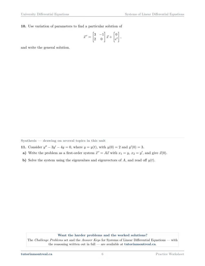
    Use variation of parameters to find a particular solution of $$\overrightarrow{x}{}^{\prime }=\left[\begin{array}{cc}3& -1\\ 2& 0\end{array}\right]\overrightarrow{x}+\left[\begin{array}{c}0\\ e^t\end{array}\right],$$ and write the general solution.

11. Q11Synthesis — drawing on several topics in this unit

    Consider $y^{″}-3y^{\prime }-4y=0$, where $y=y(t)$, with $y(0)=2$ and $y^{\prime }(0)=3$.

    1. Write the problem as a first-order system $\overrightarrow{x}{}^{\prime }=A\overrightarrow{x}$ with $x_1=y$, $x_2=y^{\prime }$, and give $\overrightarrow{x}(0)$.
    2. Solve the system using the eigenvalues and eigenvectors of $A$, and read off $y(t)$.

The 7 challenge problems for this topic are a separate, paid sheet and are not reproduced here.

How to do every concept on this sheet

This is the part worksheet sites usually leave out. Below is the actual reasoning behind each group of questions — not a full solution set, the decisions that get you to one. Read it before you start, or after you get stuck.

Writing a higher-order equation as a first-order system

Every method in this chapter works on first-order systems, so the first skill is getting there. Q1 gives a single third-order equation with initial conditions and fixes the new unknowns for you: x₁ = y, x₂ = y′, x₃ = y″. The question asks for three things — the matrix A(t), the forcing vector f⃗(t) and the initial vector x⃗(0) — and each comes from a different place.

Q2 does the same with two unknown functions, each of second order, coupled because each equation contains the other function. There is no one to choose the components for you in part (a): take one component for each unknown function and one for each of its derivatives below the highest that appears, and say in words what each one stands for. The rows then come exactly as in Q1 — definitions first, then each equation solved for its highest derivative.

Linear systems in matrix form and the general solution

For a homogeneous system x⃗′ = A x⃗ with an n × n matrix, the general solution is a combination of n solutions that are linearly independent — a fundamental set — exactly as a second-order equation needed two. Q3 hands you two candidate solutions and asks you to check all of that before using them.

Part (a) is a direct check: differentiate each vector function and compare with A times it. Both sides carry the same exponential, so the comparison reduces to a statement about a constant vector — and if you recognise that statement, you have met the eigenvalue method one sheet early.

Part (c) writes the general solution as c₁x⃗₁ + c₂x⃗₂ and then fits the initial condition. At t = 0 every exponential equals 1, so the condition becomes a 2 × 2 linear system for the constants — solve it by row reduction or Cramer's rule, then substitute the constants back into the general solution rather than stopping at their values.

Distinct real eigenvalues

Try a solution of the form x⃗ = e^(λt) v⃗ with a constant vector v⃗. Substituting and cancelling the exponential leaves A v⃗ = λ v⃗: the trial works exactly when λ is an eigenvalue of A and v⃗ an eigenvector for it. Q4 asks for the general solution of a 2 × 2 system this way.

Q5 is the same method with a 3 × 3 matrix and an initial condition. Before expanding a determinant, look at the shape of the matrix: when every entry below the diagonal is zero, the determinant of A − λI is the product of its diagonal entries, and the eigenvalues can be read off without a cubic.

Complex eigenvalues

When the characteristic polynomial has no real roots, the eigenvalues come as a conjugate pair α ± iβ with conjugate eigenvectors. The method still produces e^(λt) v⃗, but it is complex, and Q6 asks for the general real-valued solution. The way through is the same idea as complex roots of a characteristic equation for a single equation.

Q7 adds an initial condition. At t = 0 the cosines are 1 and the sines 0, so the condition again gives a small linear system for the two constants — with the vectors a⃗ and b⃗ as its columns. Different choices of eigenvector give different-looking general solutions; after the initial condition, they must all give the same function.

A repeated eigenvalue

When the characteristic polynomial has a double root, a 2 × 2 matrix may have only one independent eigenvector, and then the eigenvalue method yields only one solution. Q8 walks through that case with the eigenvalue given to you.

Part (a) is a statement about the null space of A − 2I: row reduce it and show that it has exactly one free variable, so every eigenvector is a multiple of one vector. Part (b) supplies the missing solution in the form the question states, e^(2t)(t v⃗ + w⃗), and asks you first to find w⃗ from (A − 2I) w⃗ = v⃗.

Nonhomogeneous linear systems

A forced system x⃗′ = A x⃗ + f⃗(t) has general solution x⃗ = x⃗_c + x⃗_p: the general solution of the homogeneous system plus any one particular solution, the same structure as for a single equation. The set uses the two methods you already know.

Q9 forces the system with linear functions of t and gives the trial solution: x⃗_p = t a⃗ + b⃗ with constant vectors. Substitute it, then match the coefficients of t and the constant terms separately; each match is a vector equation, so the two together are four scalar equations in the four unknown entries.

Q10 asks for variation of parameters instead. Put the two homogeneous solutions side by side as the columns of a fundamental matrix Φ(t); the particular solution is then built from Φ⁻¹ f⃗, integrated and multiplied back by Φ.

The synthesis question

Q11 closes the loop with the start of the set. Part (a) is Q1's rewriting on a second-order equation: two components, a 2 × 2 matrix and an initial vector. Part (b) solves that system by the eigenvalue method of Q4 and Q5, fits the initial condition, and then reads y(t) off as the first component — the second component should then be its derivative, which is a free check on the whole computation.

Preview all 6 pages

Click any page to open the full PDF.

Getting the most out of it

Check every eigenvector by multiplying

Computing A v⃗ and comparing it with λ v⃗ takes a few seconds, and an eigenvector error ruins everything that follows — the solutions, the constants, the initial-value fit. Make the check a reflex, including for complex eigenvectors.

Decide the case before you compute

Once the characteristic polynomial is in hand, say which case you are in — distinct real, complex pair, or repeated — before you look for eigenvectors. Each case assembles the general solution differently, and writing the template first keeps you from mixing them.

Label every component

When you convert an equation or a coupled pair to a system, write down in words what each x_k stands for. It is what lets you read the answer back — which component is y, which is its derivative — and what tells you which initial values you need.

Fit initial conditions at t = 0 with the vectors as columns

Every initial-value fit in this chapter is the same step: at t = 0 the exponentials become 1, and the constants solve a linear system whose columns are the solution vectors evaluated there. Write that augmented matrix explicitly, then row reduce.

Differentiate your answer once

A final check costs one derivative: differentiate your solution and compare it with A times it (plus the forcing, if there is one). It confirms the eigenvalues, the eigenvectors and the algebra in a single step.

Common questions